This document provides an overview of synchronous machines and synchronous condensers. It discusses key topics such as:
- The basic components and operating principles of synchronous machines and how they can function as motors or generators.
- Concepts like torque, power, energy and their relationships in synchronous machines.
- How synchronous machines synchronize to the frequency of the power system and their operating speed relationship.
- Power flow, internal and terminal voltages, and torque angle in synchronous machines.
- Losses that occur in synchronous machines and how efficiency is affected.
- The use of synchronous condensers to provide reactive power support through field excitation control while transferring little to no real power.
- Models for analyzing
Overview and introduction to synchronous machines course by Heydt, Kalsi, and Kyriakides.
Discusses the basic principles of synchronous machines; generation, motor functions, stator and rotor structure, and torque-speed relationships.
Examines AC power flow, voltage relationships, and conditions for generator and motor action in synchronous machines.
Examples calculating output power, phase angle effects, and implications for active power in synchronous generator applications. Explains power factor in relation to voltages, currents, and machine operations, emphasizing controllability through excitation.
Describes synchronous condenser operations emphasizing reactive power, voltage support and power factor correction capabilities.
Introduces modeling techniques for synchronous machines, saturation effects, and transients in electrical circuits.
Basics of state estimation, matrix techniques for handling measurements, including real power and voltage estimations.
Implements Digital Fault Recorders for performance monitoring during stressed conditions and illustrates torque angle calculations.
Opens the floor for questions and answers regarding the presented material on synchronous machines and state estimation.
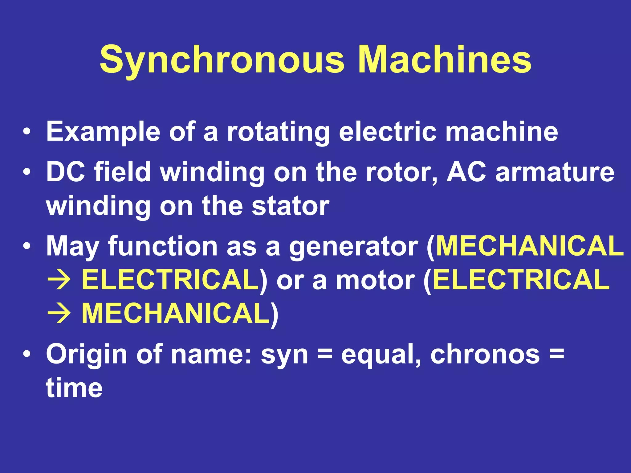
Synchronous Machines
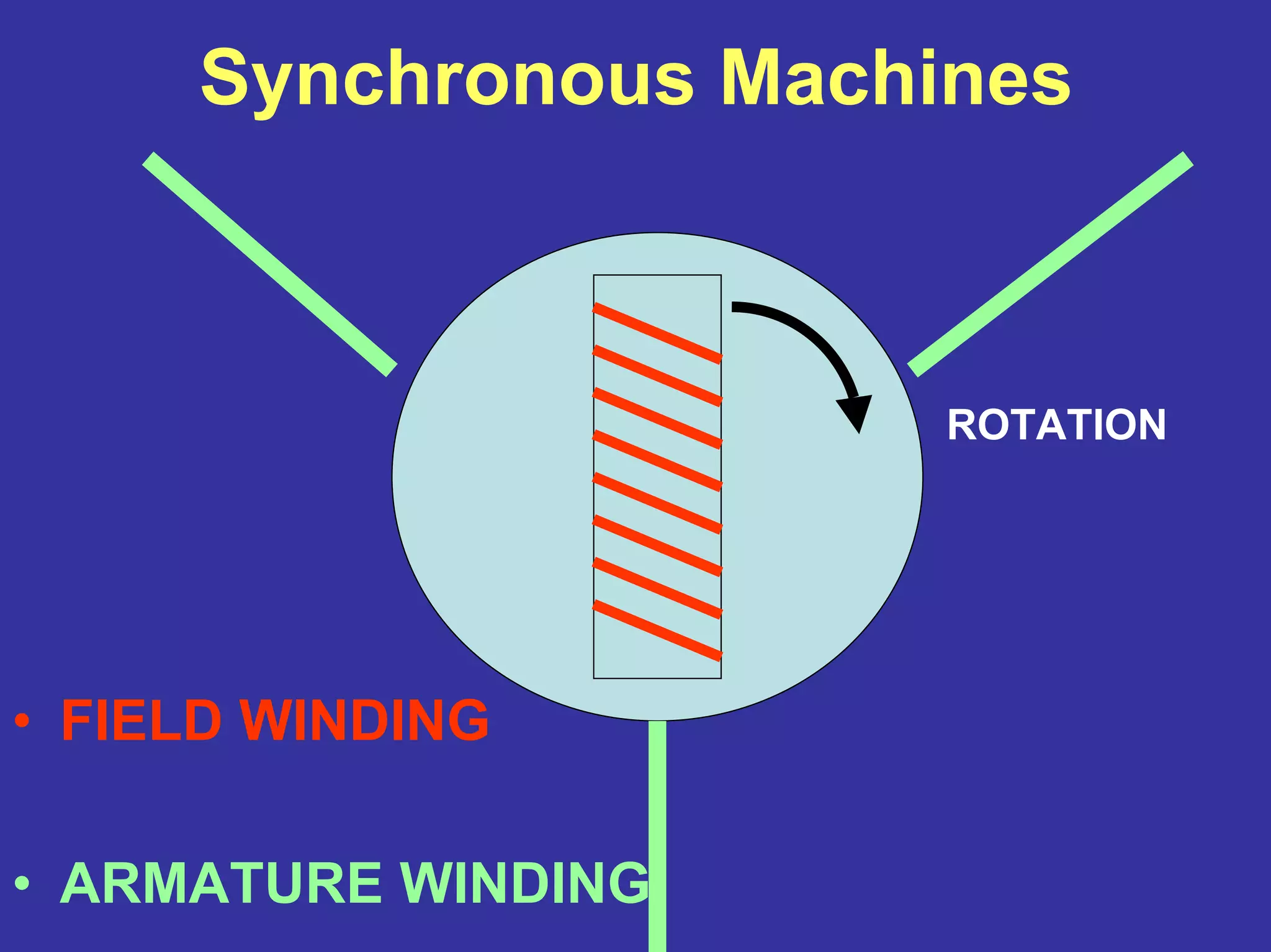
• Exampleof a rotating electric machine
• DC field winding on the rotor, AC armature
winding on the stator
• May function as a generator (MECHANICAL
ELECTRICAL) or a motor (ELECTRICAL
MECHANICAL)
• Origin of name: syn = equal, chronos =
time
Synchronous Machines
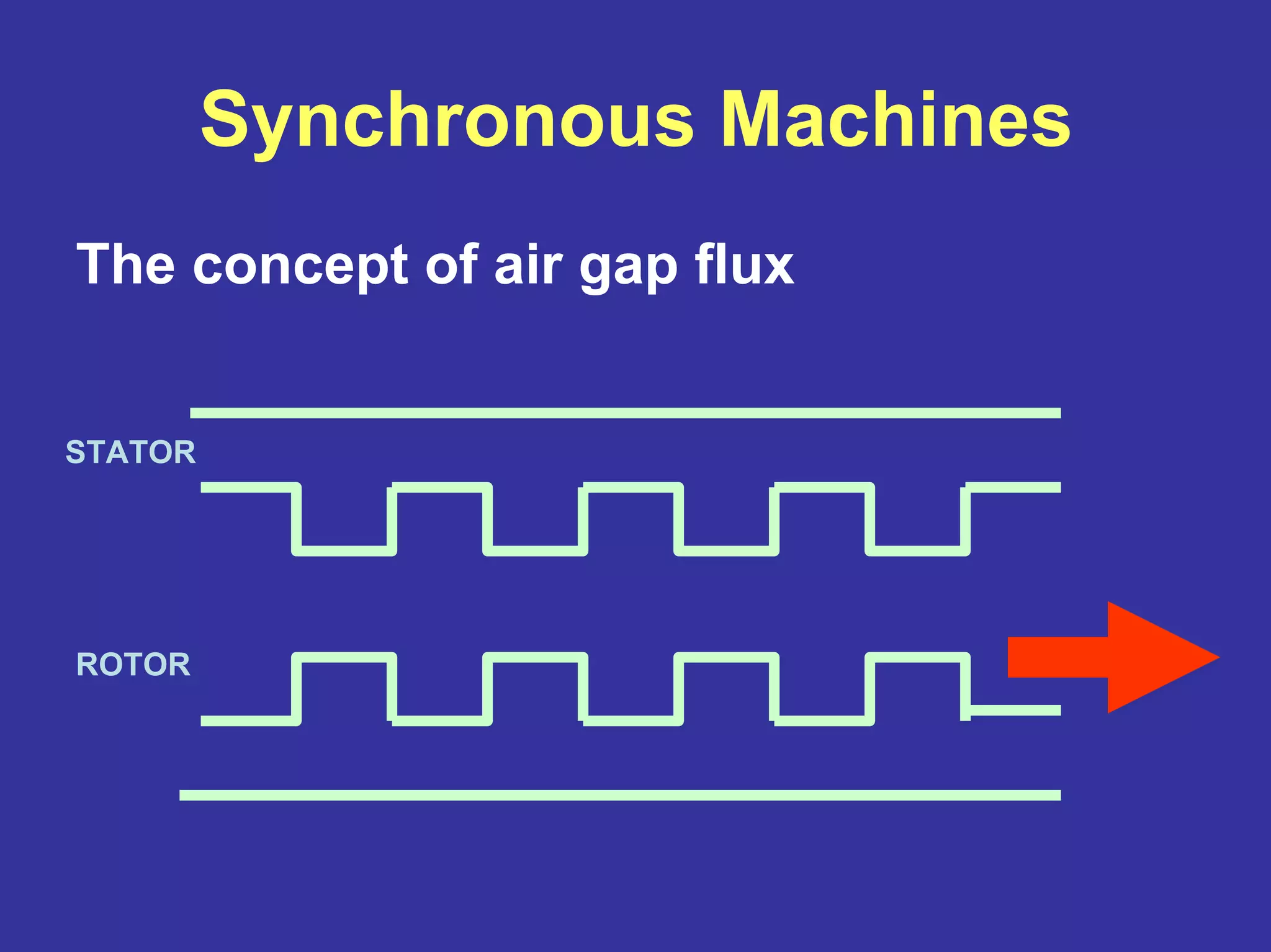
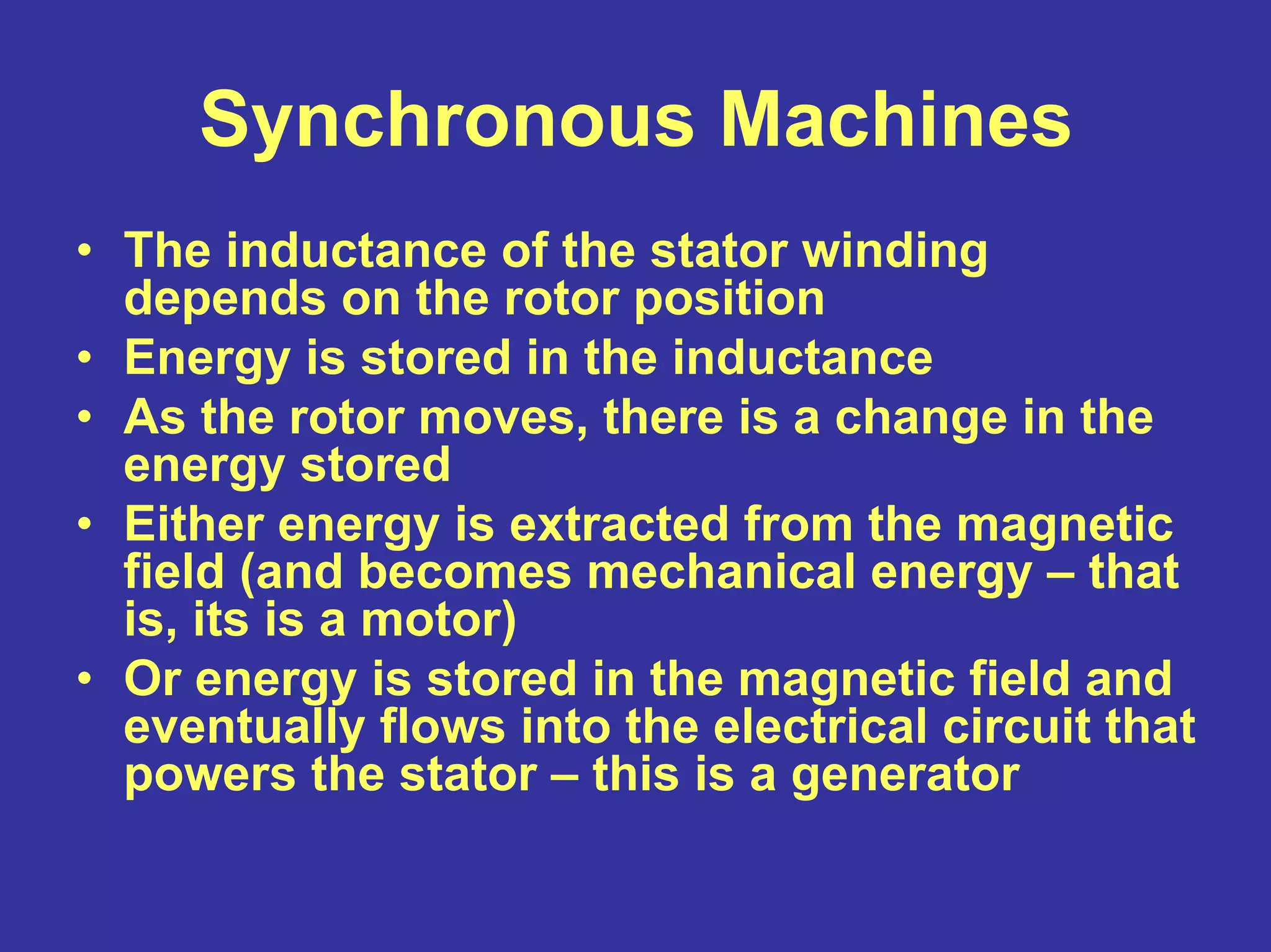
• Theinductance of the stator winding
depends on the rotor position
• Energy is stored in the inductance
• As the rotor moves, there is a change in the
energy stored
• Either energy is extracted from the magnetic
field (and becomes mechanical energy – that
is, its is a motor)
• Or energy is stored in the magnetic field and
eventually flows into the electrical circuit that
powers the stator – this is a generator
7.
Synchronous Machines
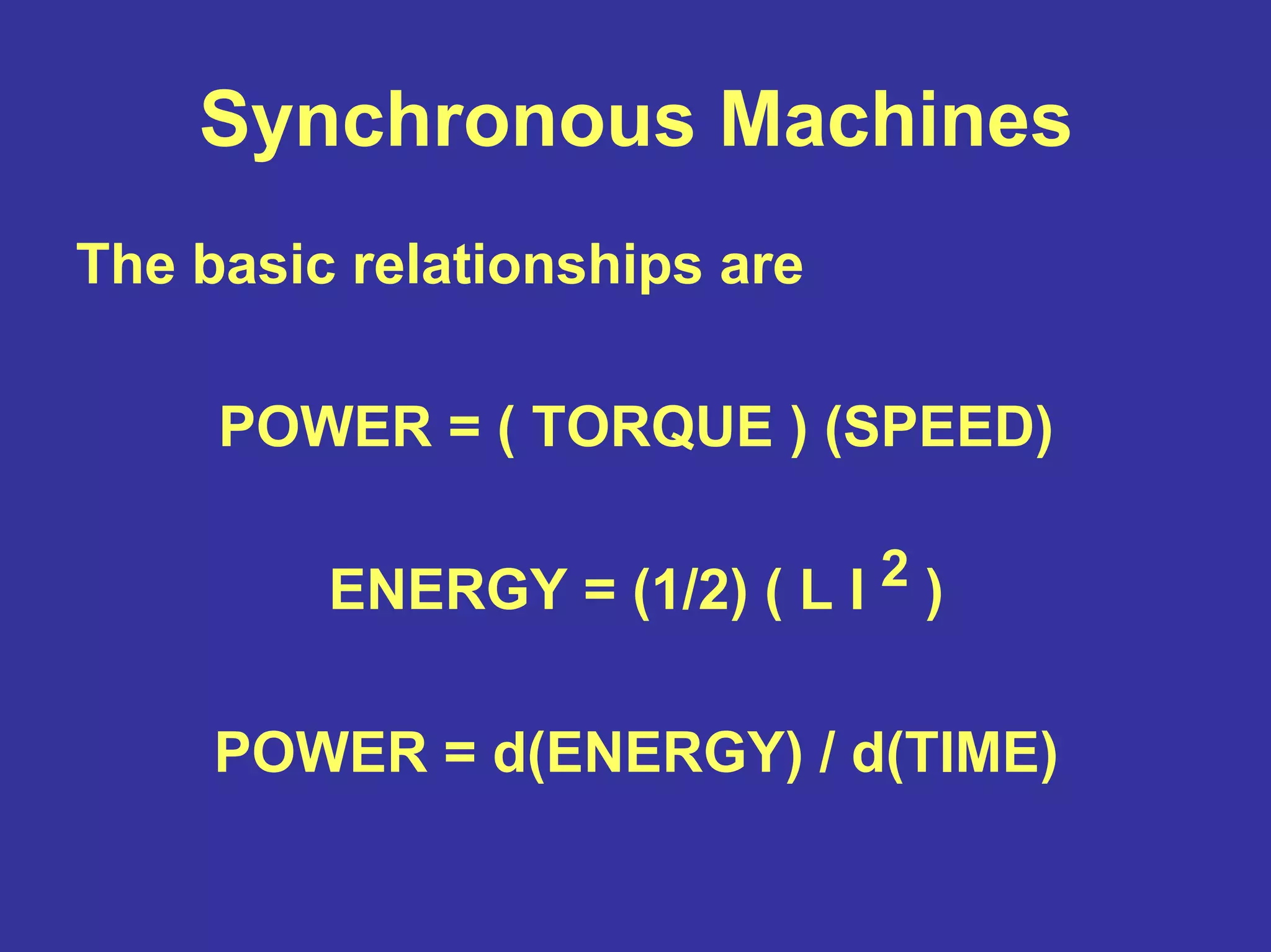
The basicrelationships are
POWER = ( TORQUE ) (SPEED)
ENERGY = (1/2) ( L I 2 )
POWER = d(ENERGY) / d(TIME)
8.
Synchronous Machines
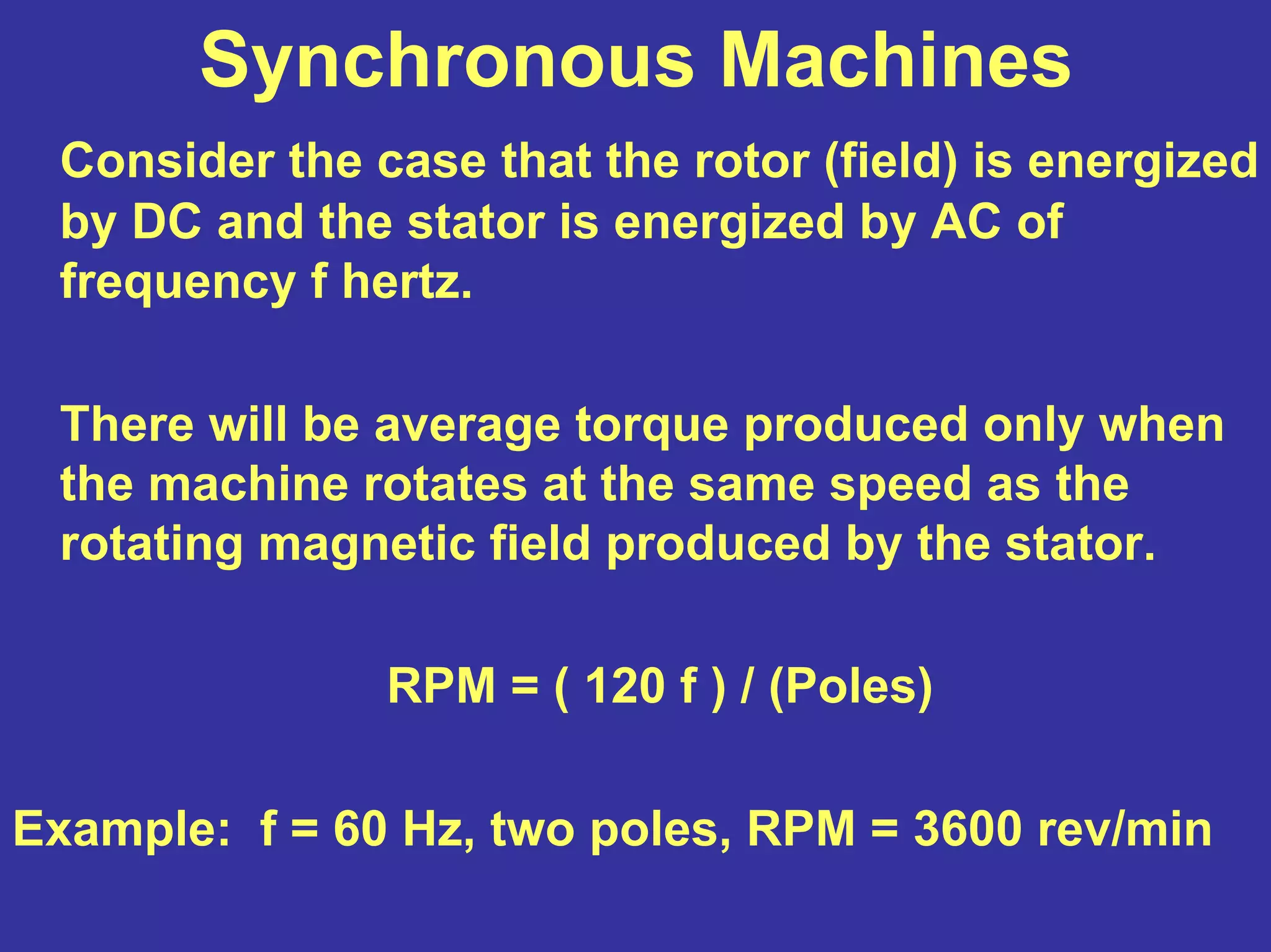
Consider thecase that the rotor (field) is energized
by DC and the stator is energized by AC of
frequency f hertz.
There will be average torque produced only when
the machine rotates at the same speed as the
rotating magnetic field produced by the stator.
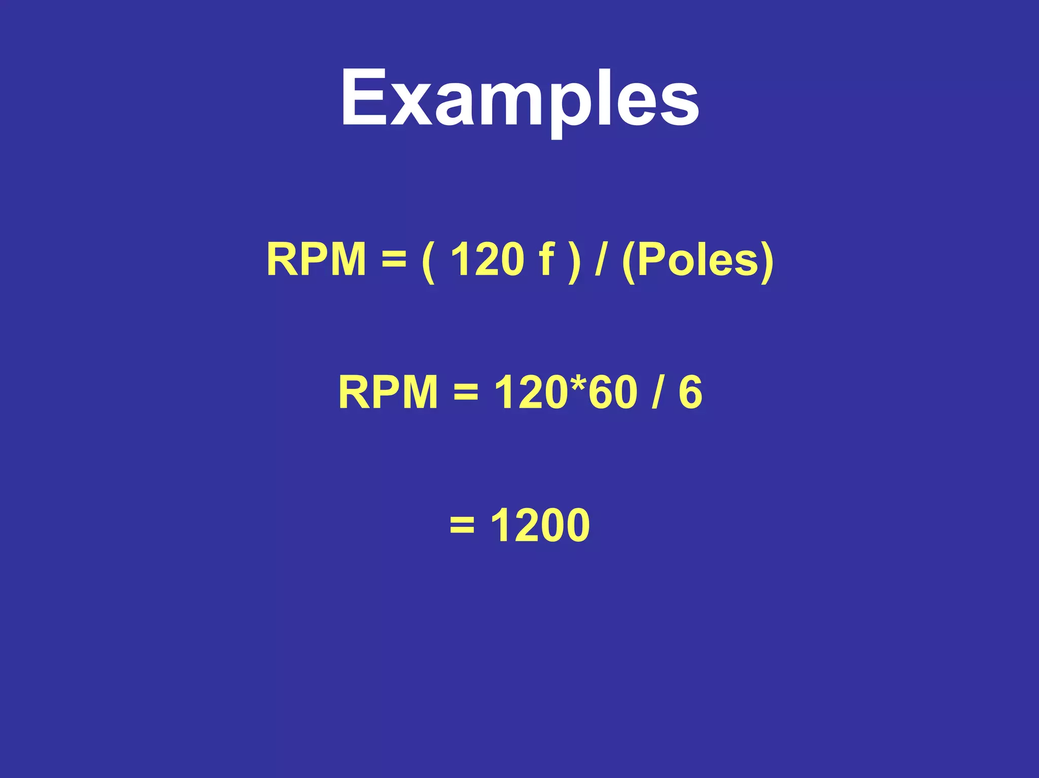
RPM = ( 120 f ) / (Poles)
Example: f = 60 Hz, two poles, RPM = 3600 rev/min
9.
Synchronous Machines
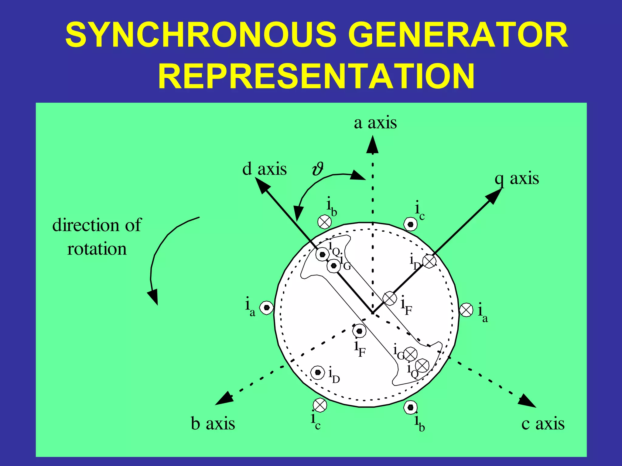
ROTATION
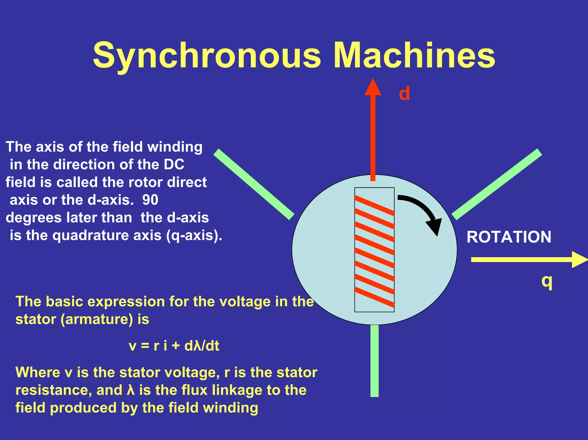
The axisof the field winding
in the direction of the DC
field is called the rotor direct
axis or the d-axis. 90
degrees later than the d-axis
is the quadrature axis (q-axis).
d
q
The basic expression for the voltage in the
stator (armature) is
v = r i + dλ/dt
Where v is the stator voltage, r is the stator
resistance, and λ is the flux linkage to the
field produced by the field winding
Synchronous Machines
Vinternal
Vterminal
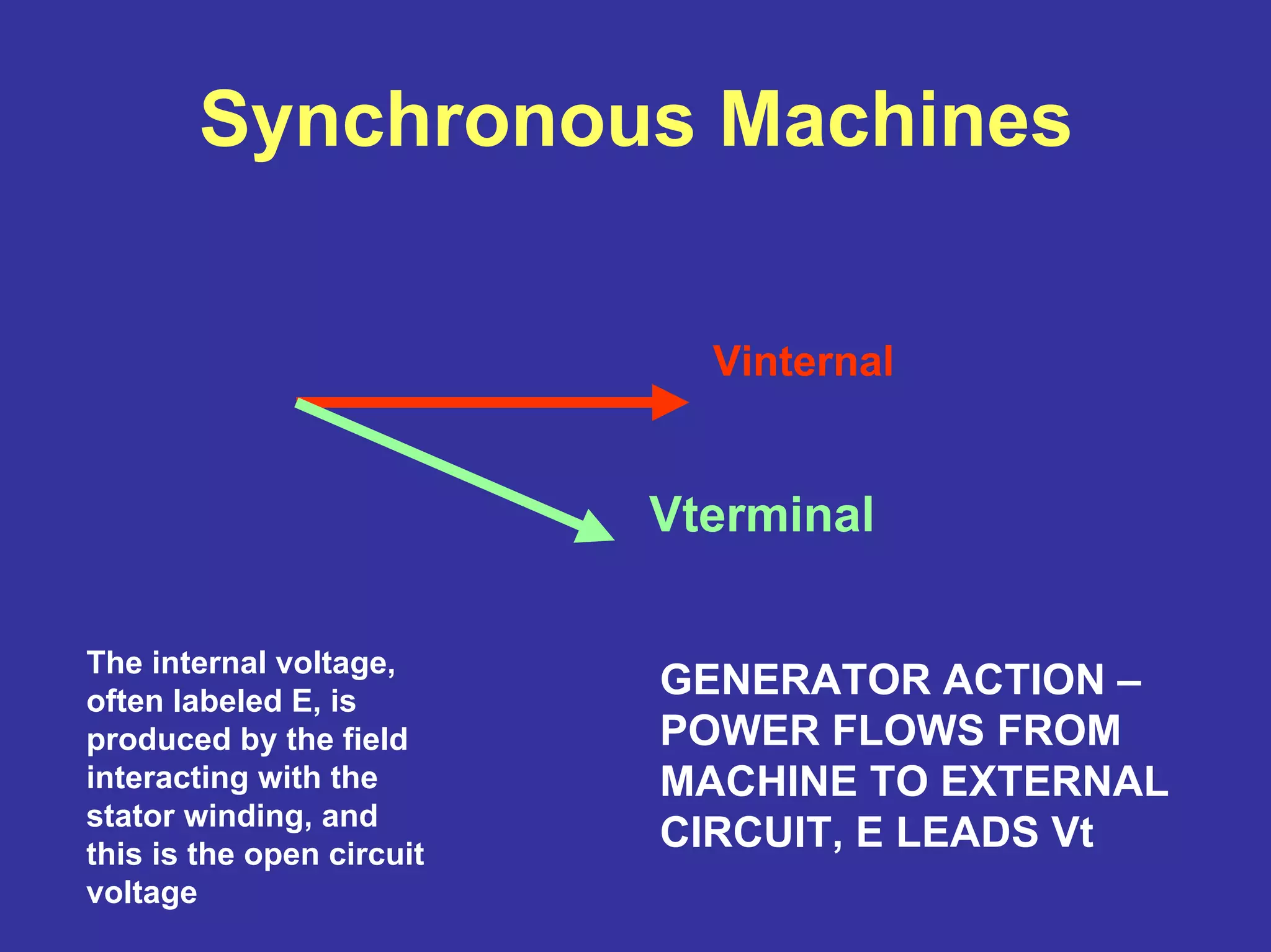
The internalvoltage,
often labeled E, is
produced by the field
interacting with the
stator winding, and
this is the open circuit
voltage
GENERATOR ACTION –
POWER FLOWS FROM
MACHINE TO EXTERNAL
CIRCUIT, E LEADS Vt
12.
Synchronous Machines
Vinternal
Vterminal
The internalvoltage,
often labeled E, is
produced by the field
interacting with the
stator winding, and
this is the open circuit
voltage
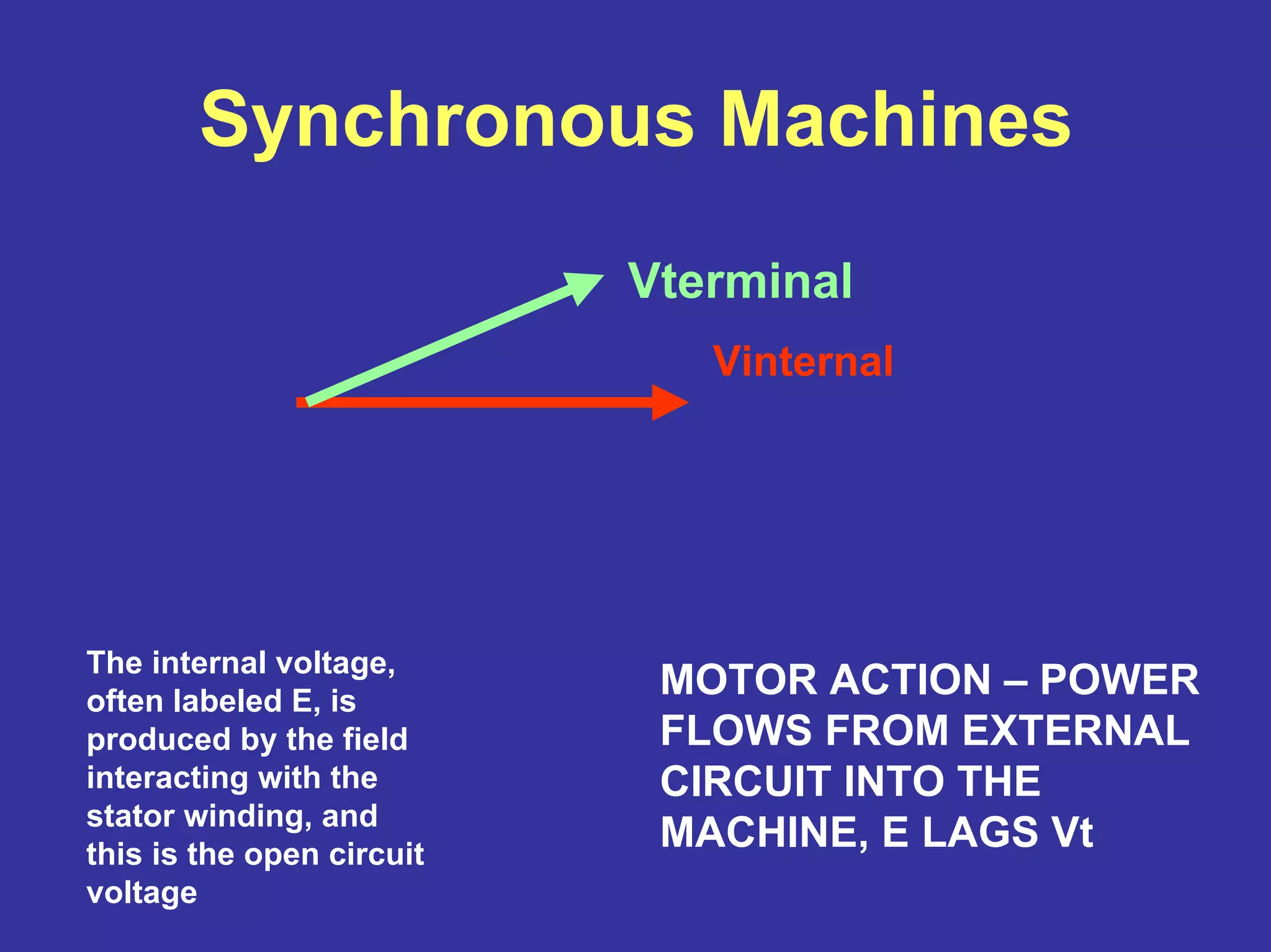
MOTOR ACTION – POWER
FLOWS FROM EXTERNAL
CIRCUIT INTO THE
MACHINE, E LAGS Vt
13.
Synchronous Machines
Vinternal =E
Vterminal = Vt
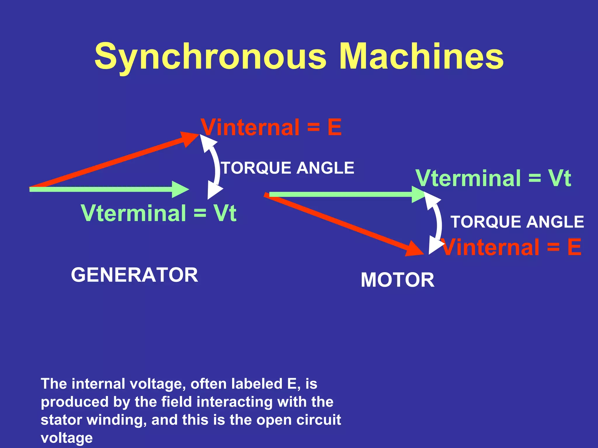
The internal voltage, often labeled E, is
produced by the field interacting with the
stator winding, and this is the open circuit
voltage
MOTOR
Vinternal = E
GENERATOR
Vterminal = Vt
TORQUE ANGLE
TORQUE ANGLE
14.
Synchronous Machines
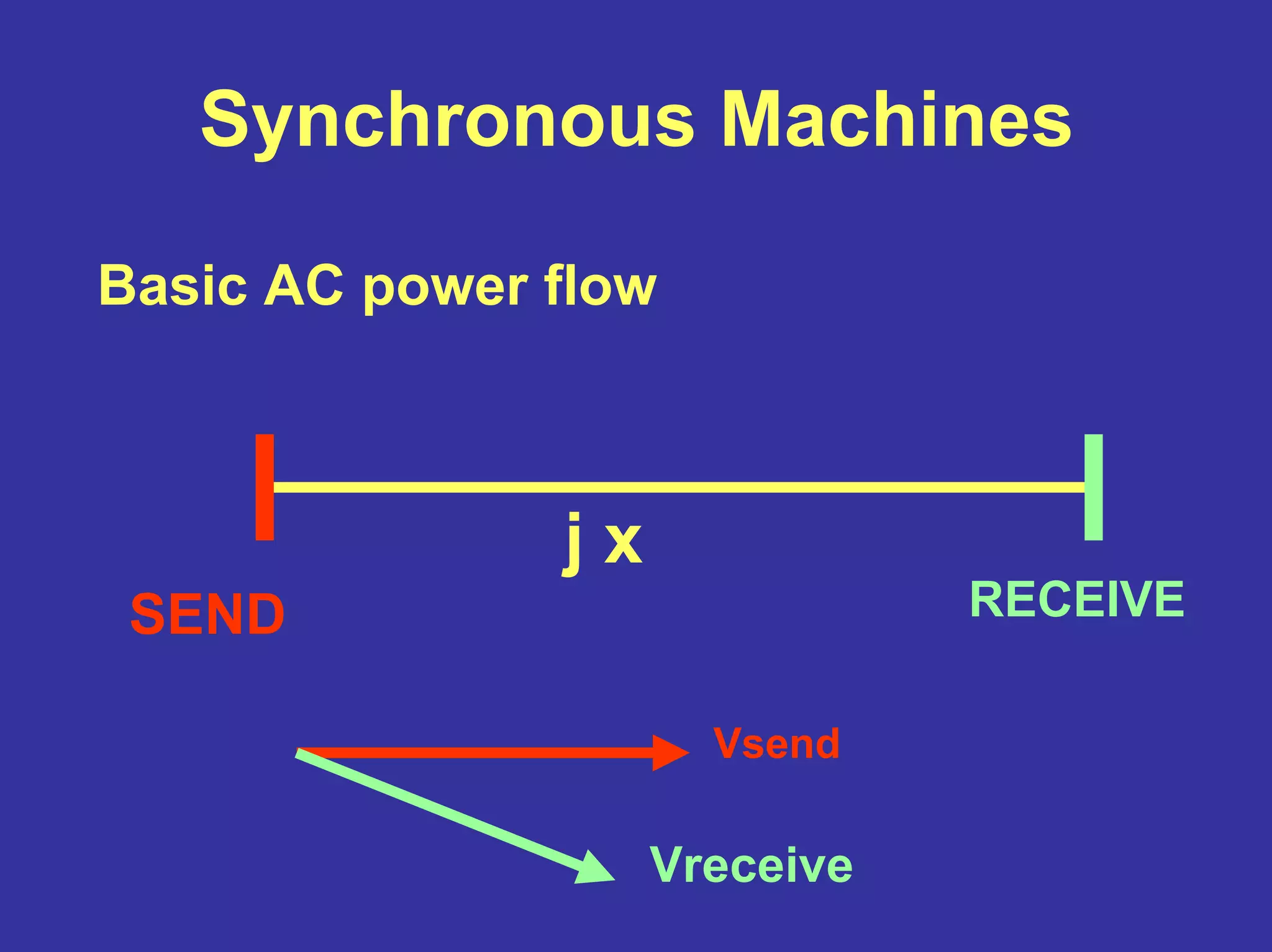
Active powerwill flow when there is a phase
difference between Vsend and Vreceive.
This is because when there is a phase
difference, there will be a voltage difference
across the reactance jx, and therefore there
will be a current flowing in jx. After some
arithmetic
Psent = [|Vsend|] [|Vreceive|] sin(torque angle) / x
15.
Synchronous Machines
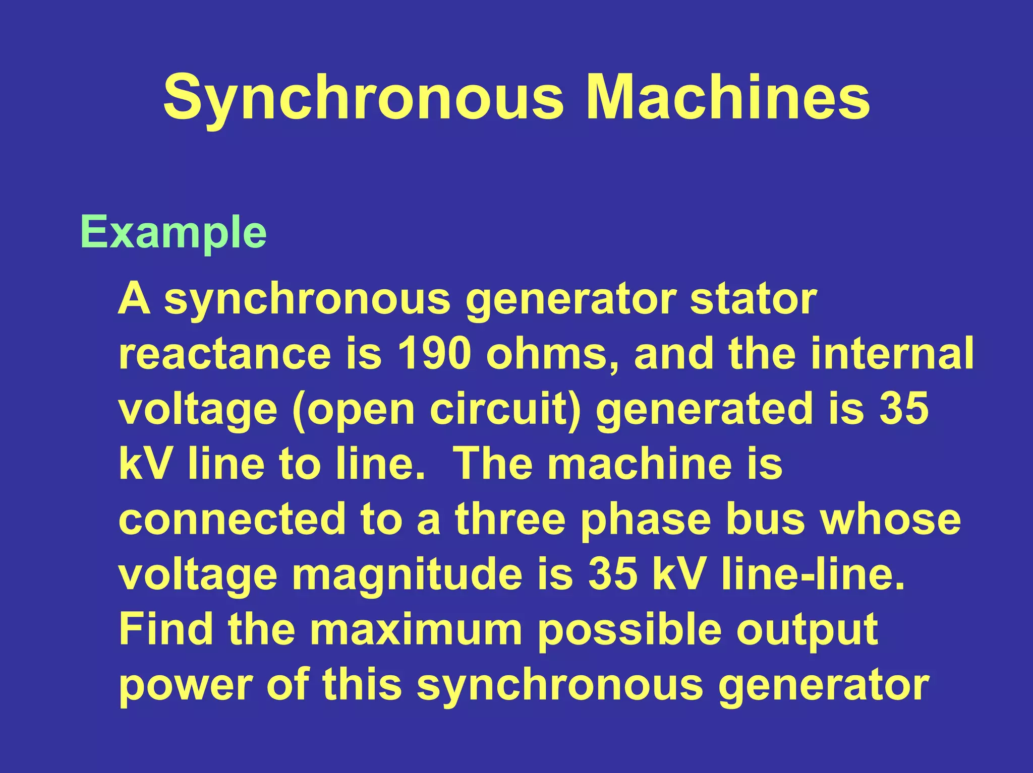
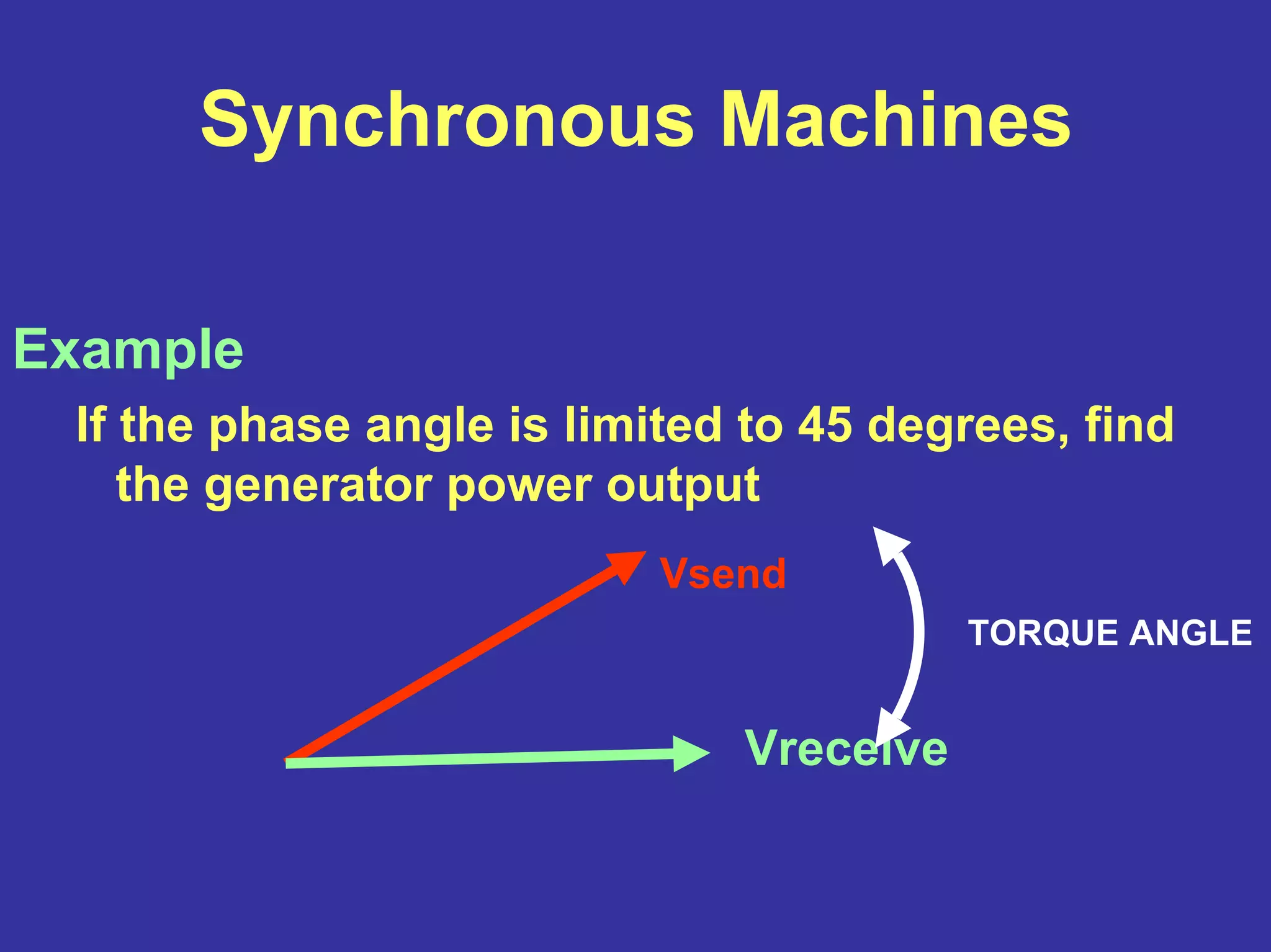
Example
A synchronousgenerator stator
reactance is 190 ohms, and the internal
voltage (open circuit) generated is 35
kV line to line. The machine is
connected to a three phase bus whose
voltage magnitude is 35 kV line-line.
Find the maximum possible output
power of this synchronous generator
16.
Synchronous Machines
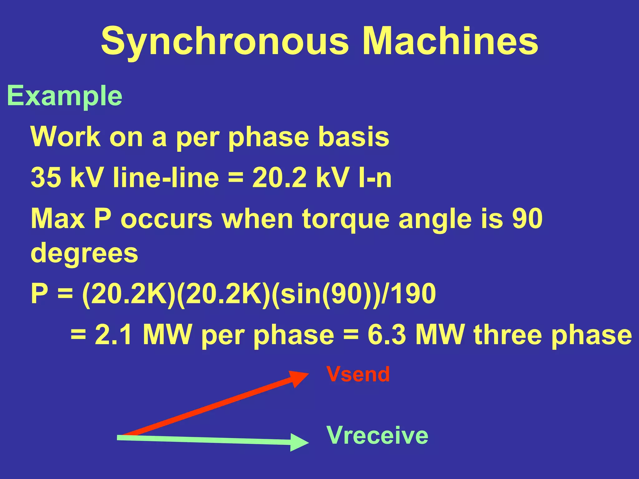
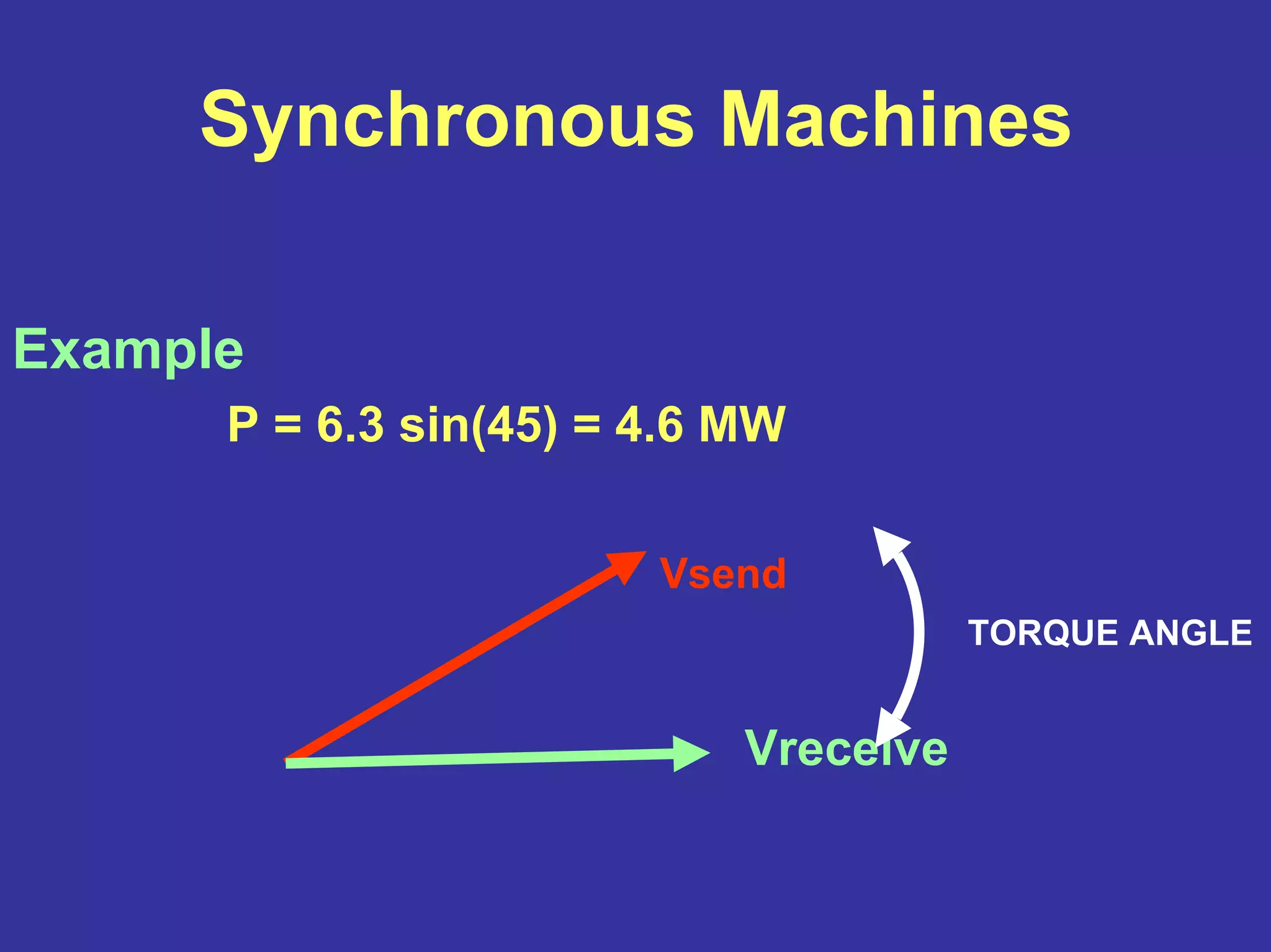
Example
Work ona per phase basis
35 kV line-line = 20.2 kV l-n
Max P occurs when torque angle is 90
degrees
P = (20.2K)(20.2K)(sin(90))/190
= 2.1 MW per phase = 6.3 MW three phase
Vsend
Vreceive
Synchronous Machines
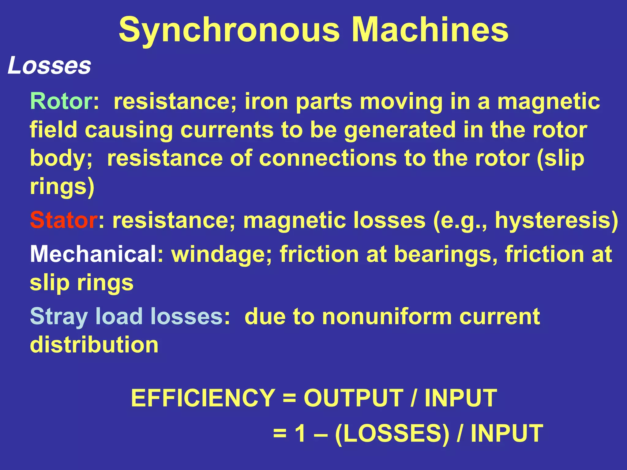
Losses
Rotor: resistance;iron parts moving in a magnetic
field causing currents to be generated in the rotor
body; resistance of connections to the rotor (slip
rings)
Stator: resistance; magnetic losses (e.g., hysteresis)
Mechanical: windage; friction at bearings, friction at
slip rings
Stray load losses: due to nonuniform current
distribution
EFFICIENCY = OUTPUT / INPUT
= 1 – (LOSSES) / INPUT
20.
Synchronous Machines
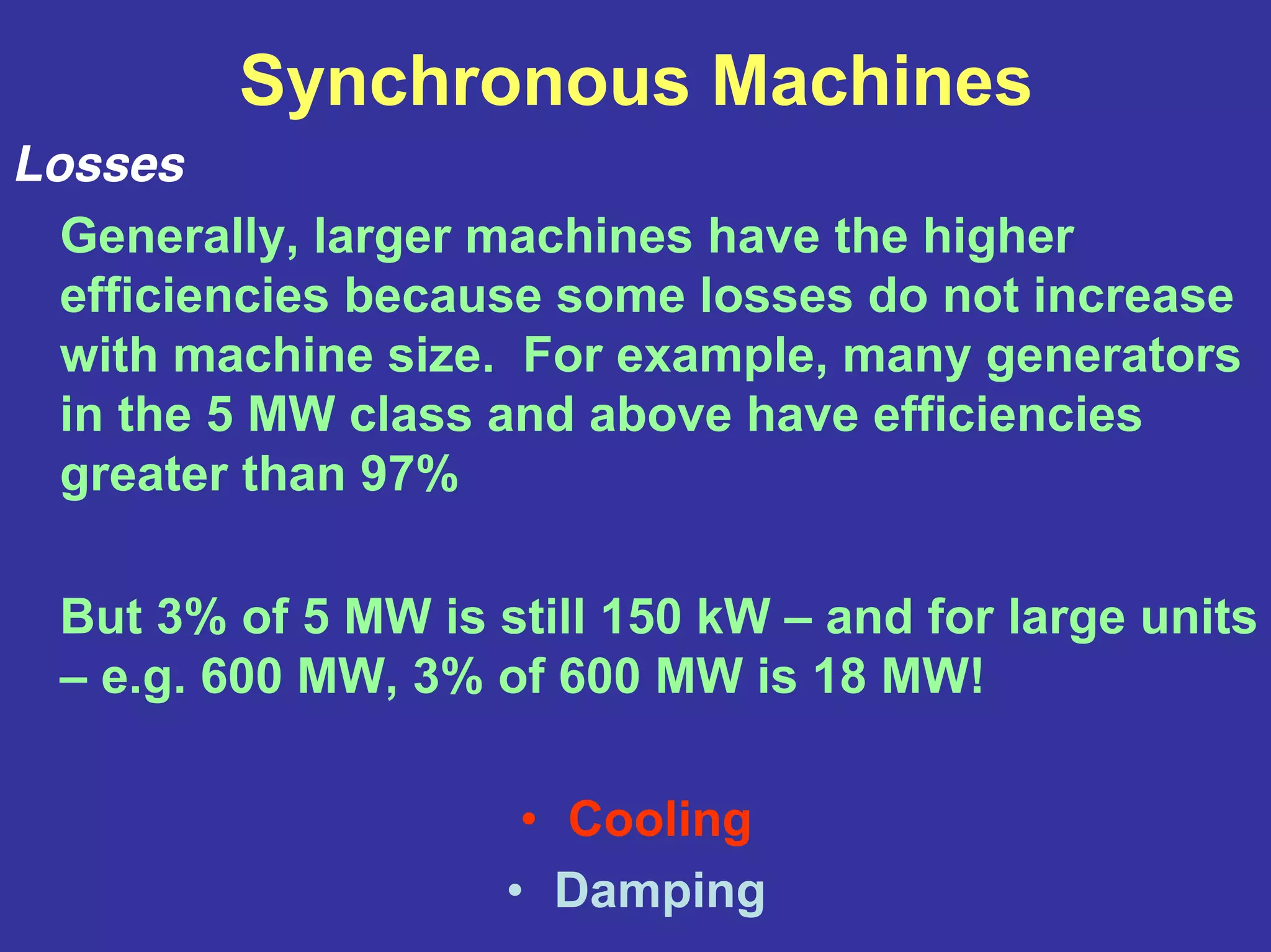
Losses
Generally, largermachines have the higher
efficiencies because some losses do not increase
with machine size. For example, many generators
in the 5 MW class and above have efficiencies
greater than 97%
But 3% of 5 MW is still 150 kW – and for large units
– e.g. 600 MW, 3% of 600 MW is 18 MW!
• Cooling
• Damping
21.
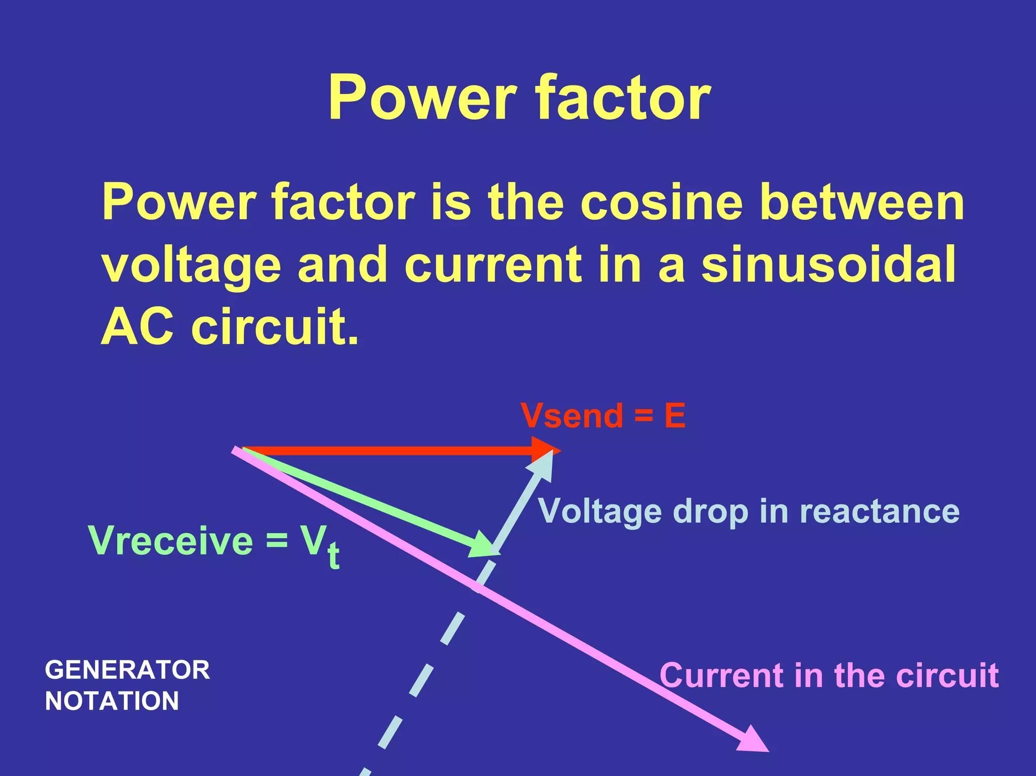
Power factor
Power factoris the cosine between
voltage and current in a sinusoidal
AC circuit.
Vsend = E
Vreceive = Vt
Voltage drop in reactance
Current in the circuitGENERATOR
NOTATION
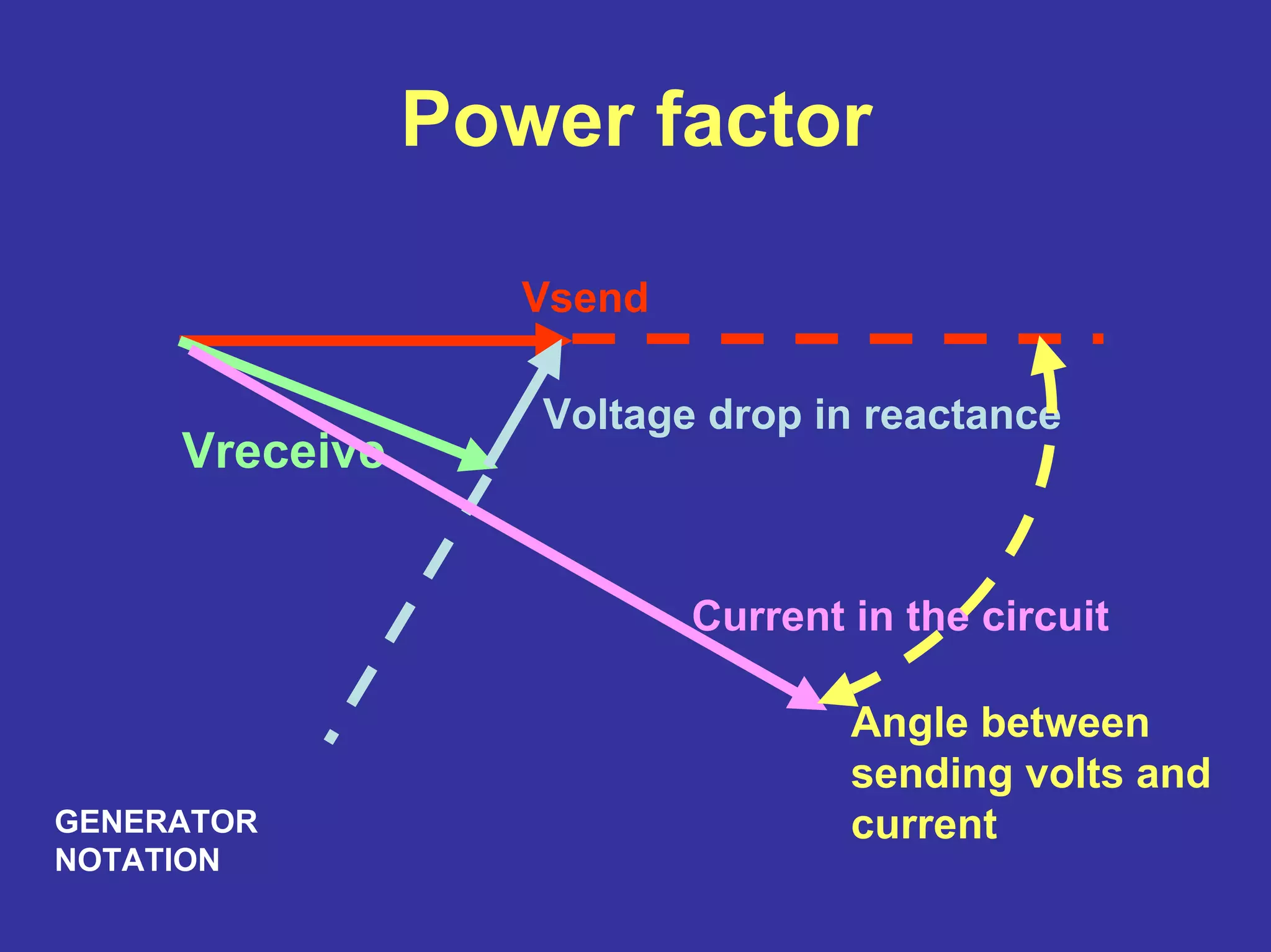
Power factor
Vsend =E
Vreceive = Vt
Voltage drop in reactance
Current in the circuit
Angle between
receiving volts and
currentCOSINE OF THIS ANGLE IS
THE MACHINE POWER
FACTOR AT THE TERMINALS
GENERATOR
NOTATION
24.
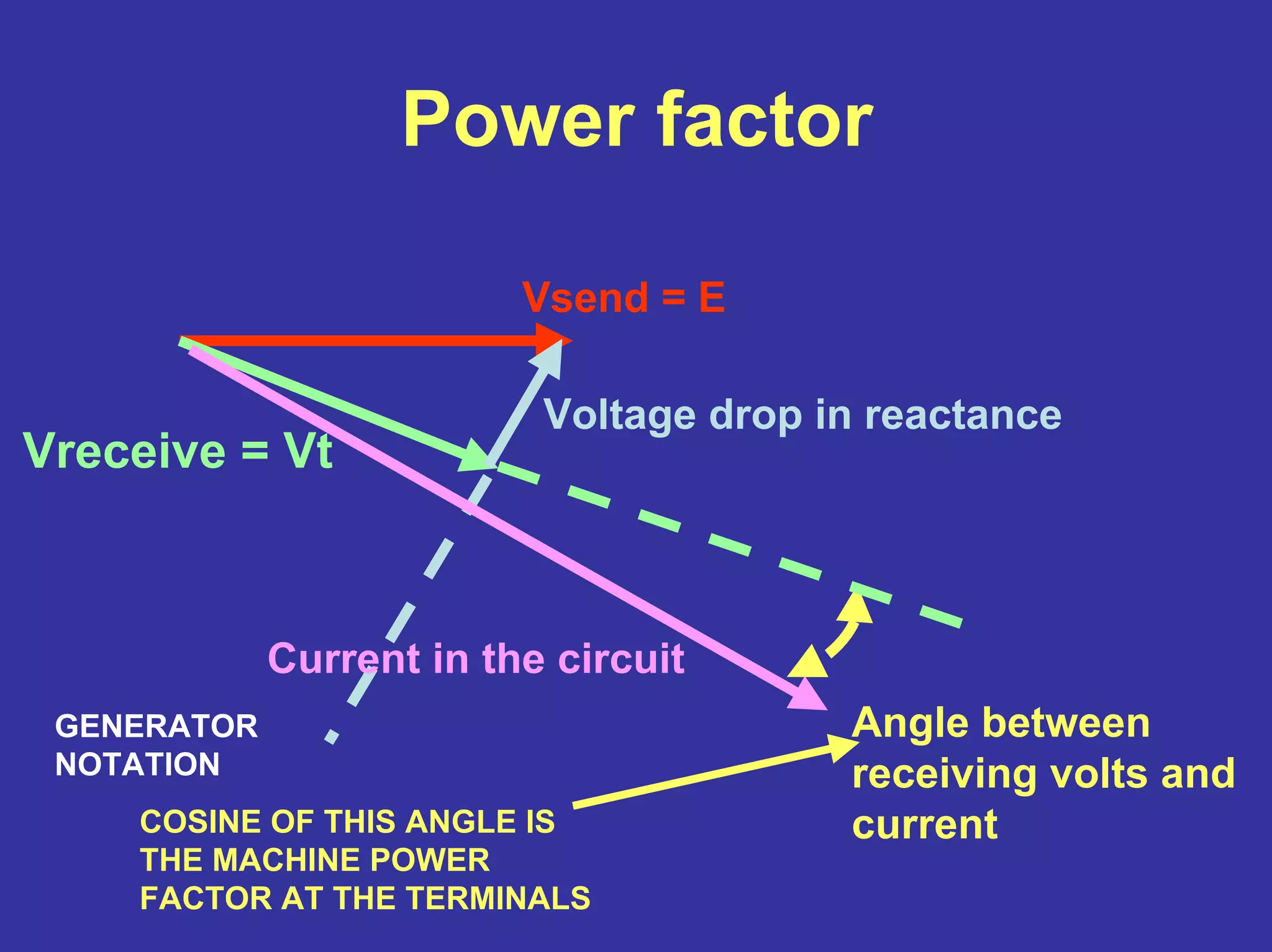
Power factor
Vsend =E
Vreceive = Vt
Voltage drop in reactance
Current in the circuit
Angle between
receiving volts
and current
COSINE OF THIS ANGLE IS
THE MACHINE POWER
FACTOR AT THE TERMINALS
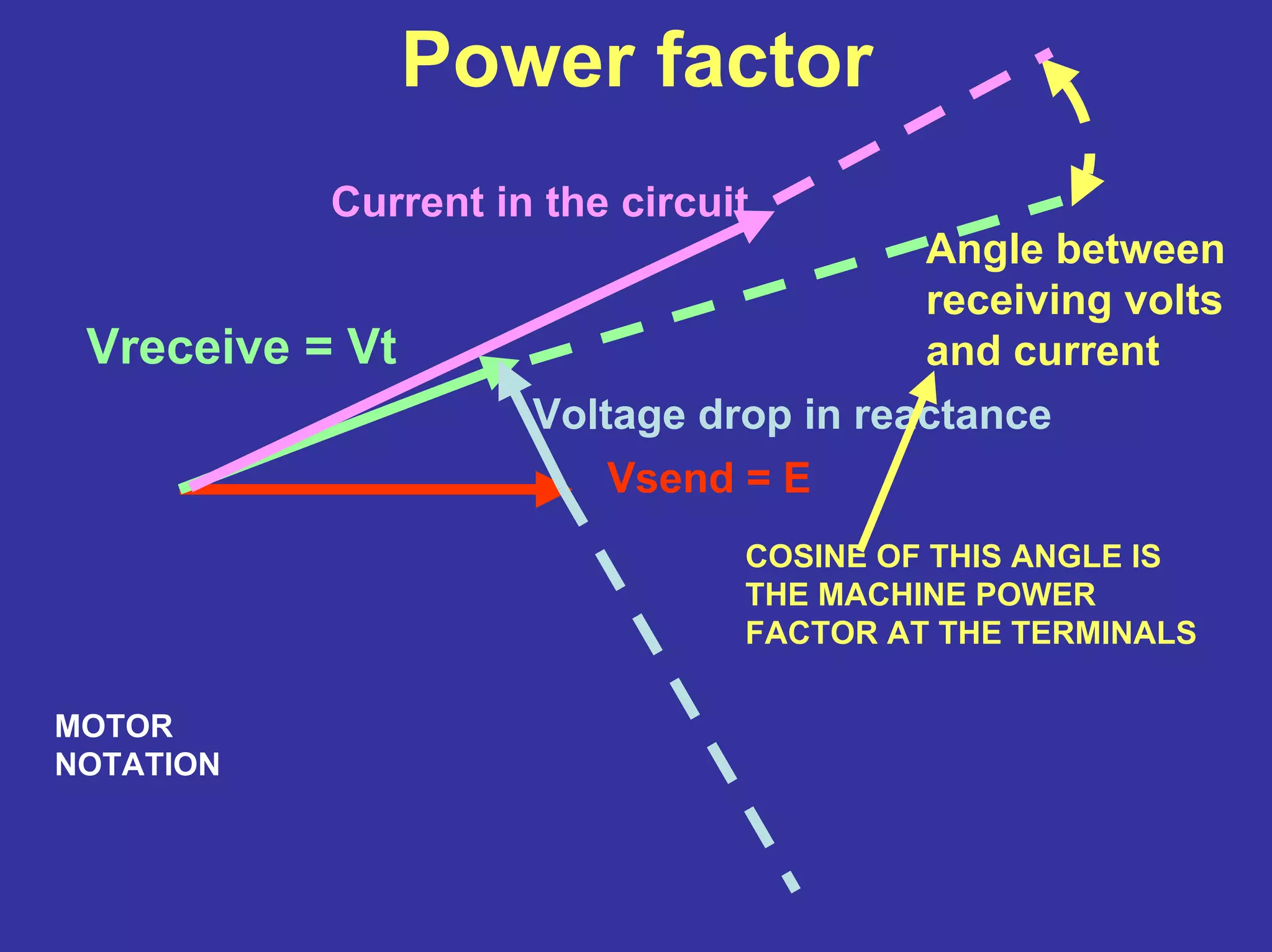
MOTOR
NOTATION
25.
Power factor
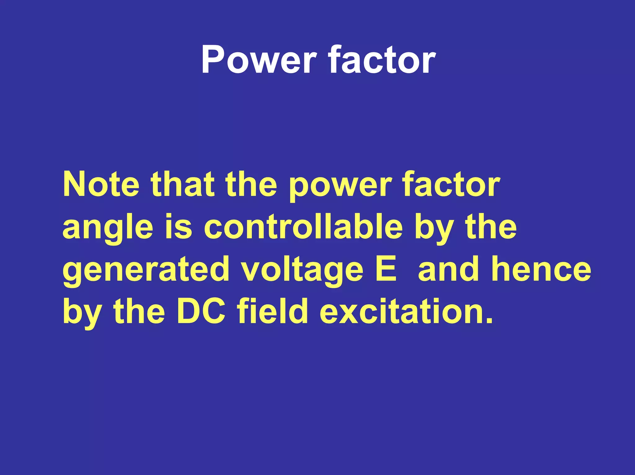
Note thatthe power factor
angle is controllable by the
generated voltage E and hence
by the DC field excitation.
Power factor
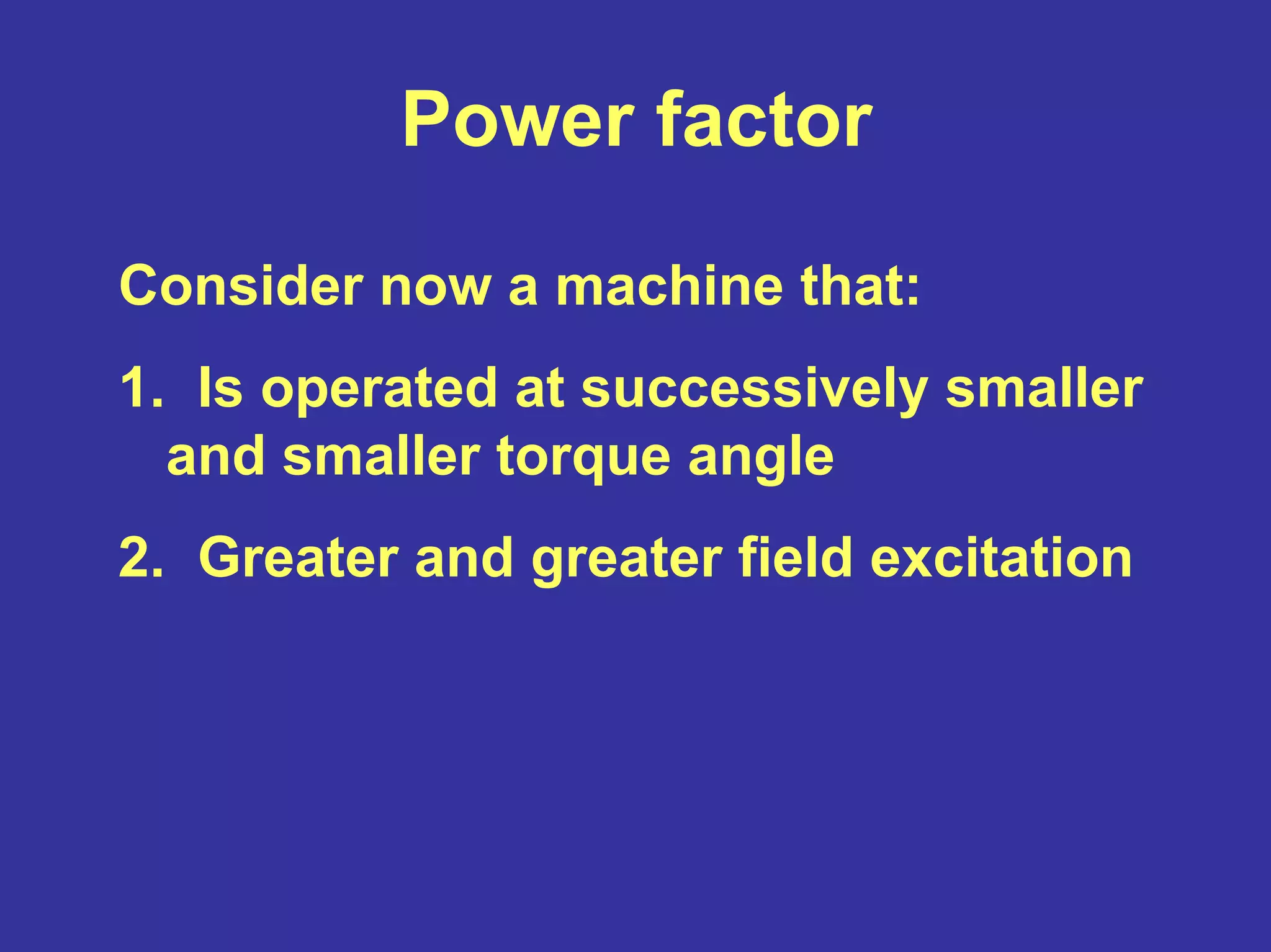
Consider nowa machine that:
1. Is operated at successively smaller
and smaller torque angle
2. Greater and greater field excitation
28.
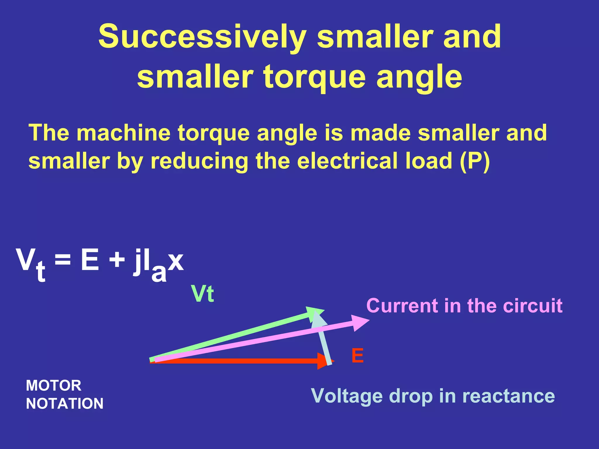
Successively smaller and
smallertorque angle
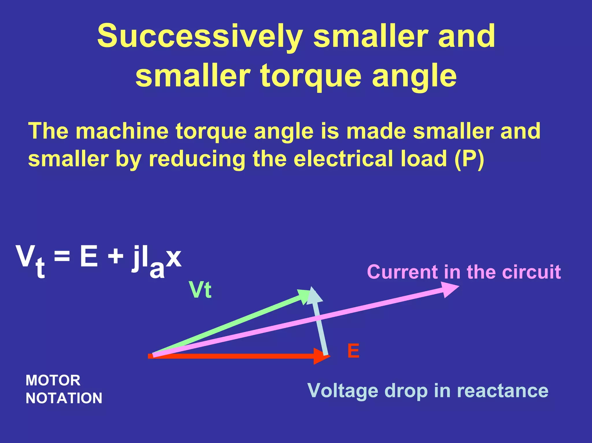
The machine torque angle is made smaller and
smaller by reducing the electrical load (P)
E
Vt
Voltage drop in reactance
Current in the circuit
MOTOR
NOTATION
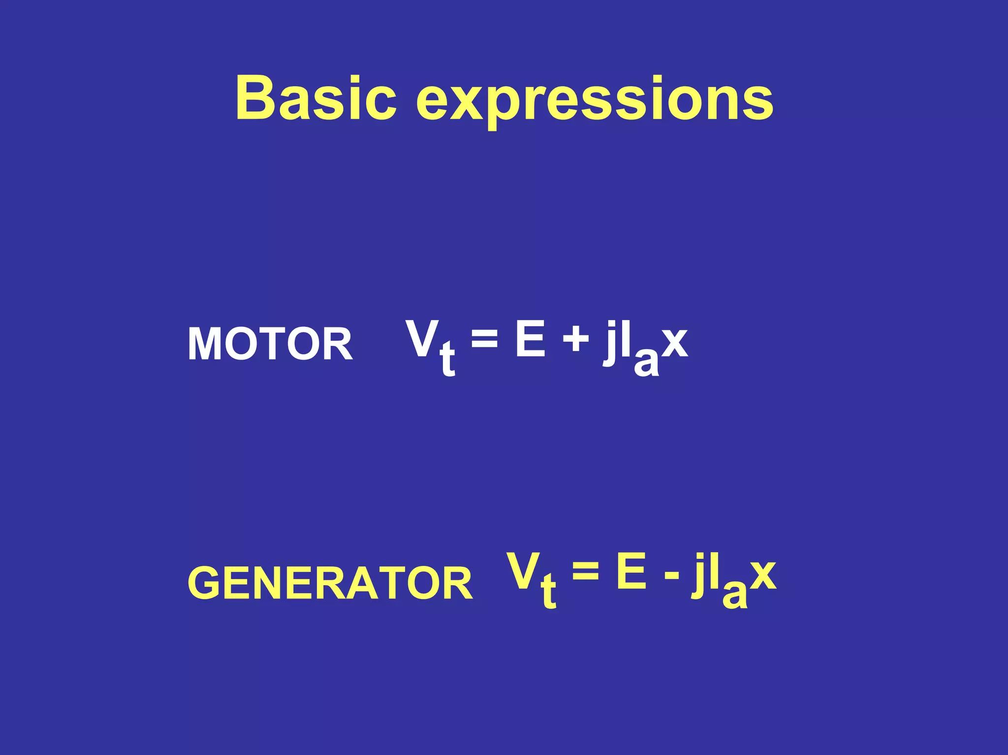
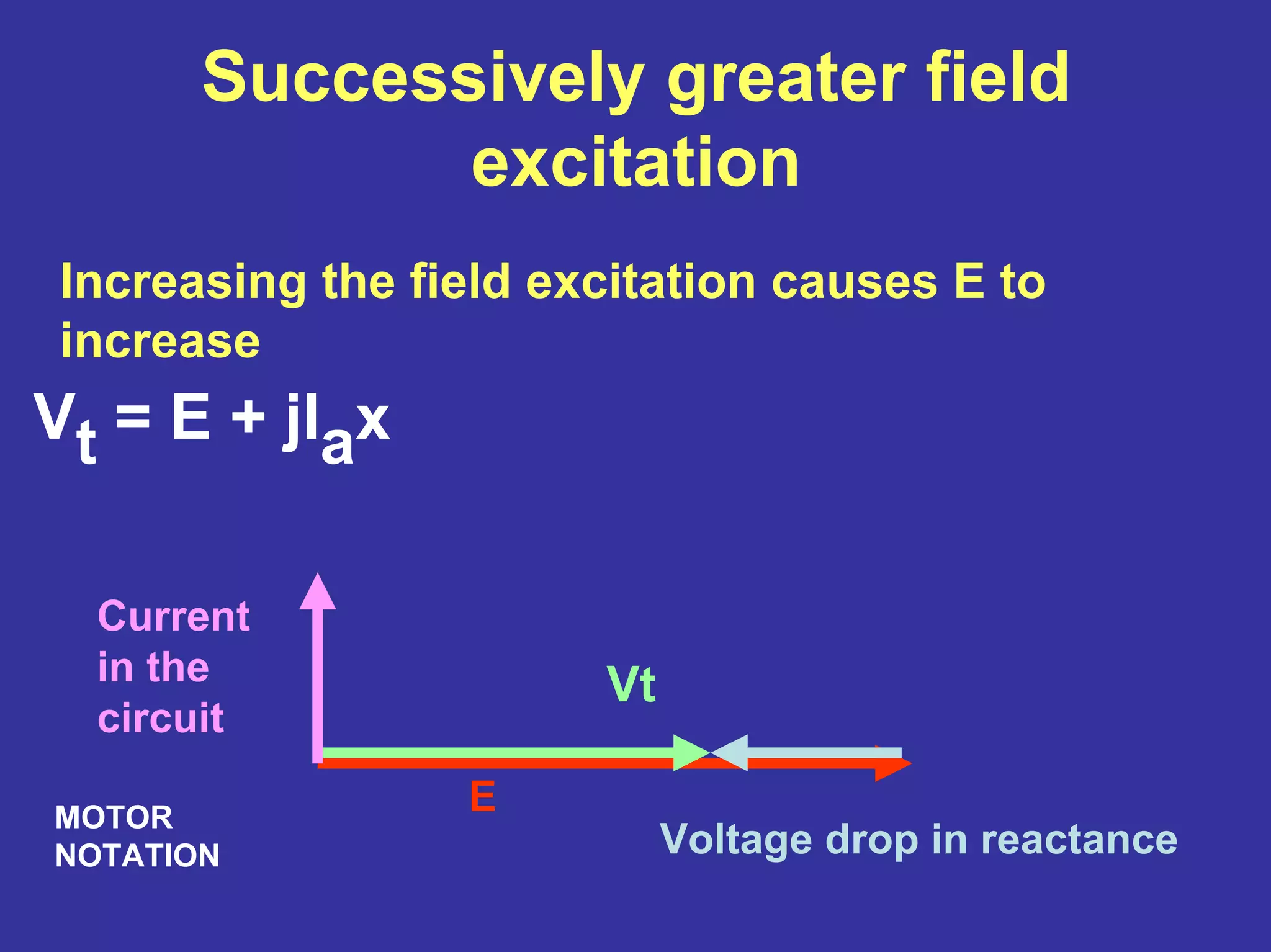
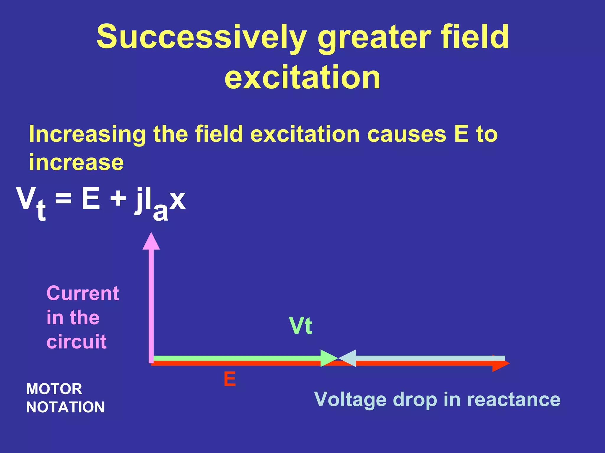
Vt = E + jIax
29.
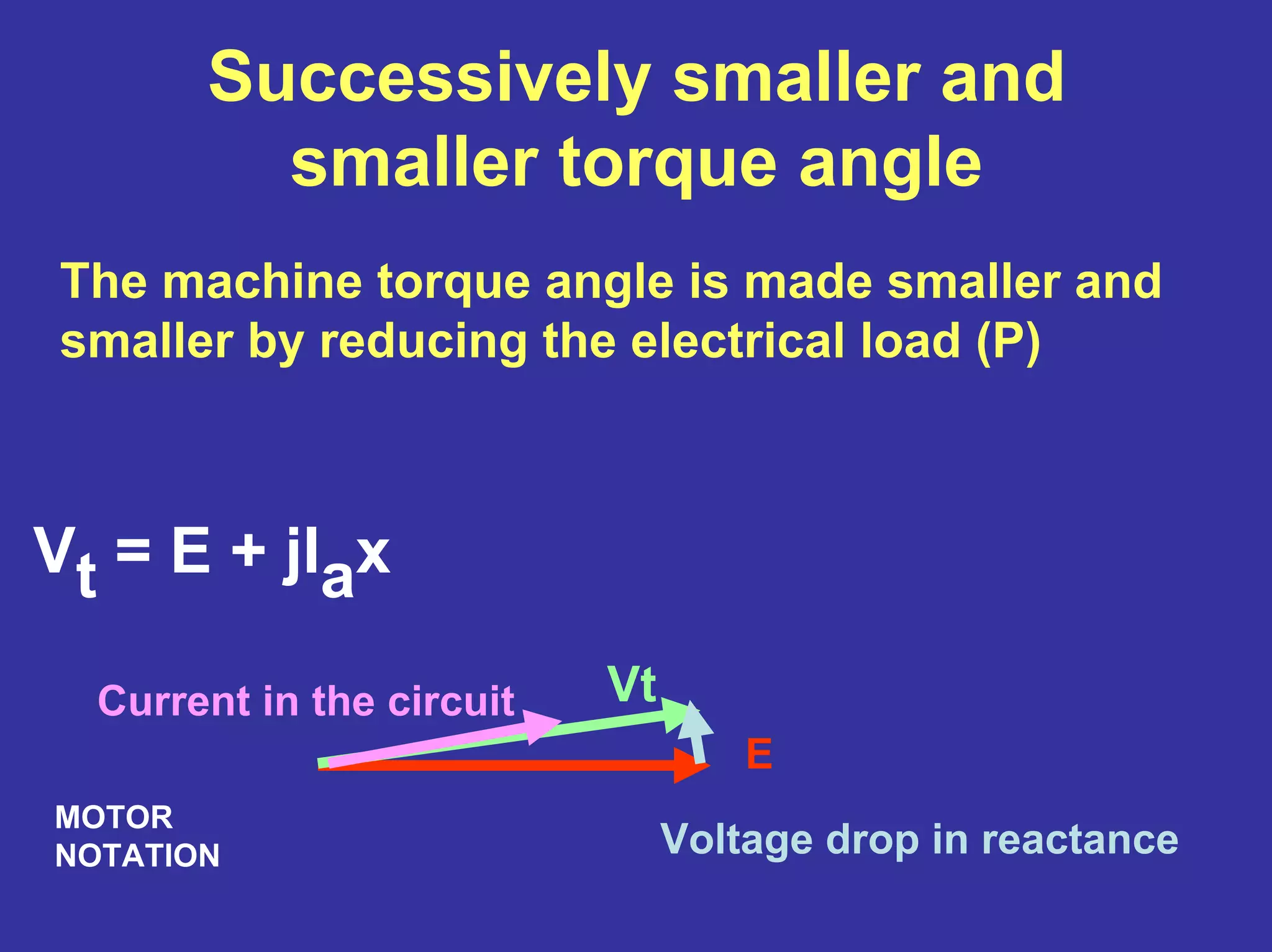
Successively smaller and
smallertorque angle
The machine torque angle is made smaller and
smaller by reducing the electrical load (P)
E
Vt
Voltage drop in reactance
Current in the circuit
MOTOR
NOTATION
Vt = E + jIax
30.
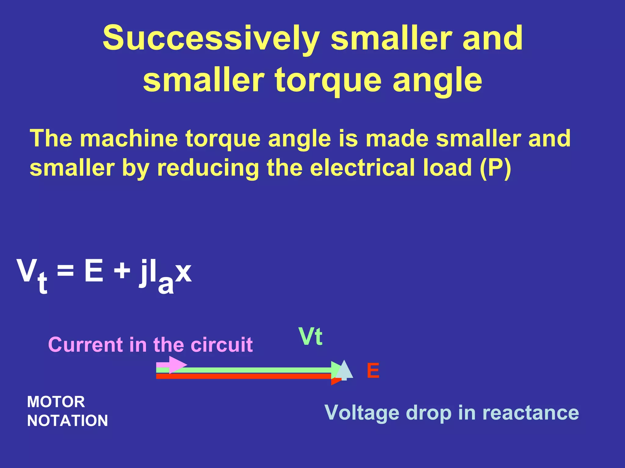
Successively smaller and
smallertorque angle
The machine torque angle is made smaller and
smaller by reducing the electrical load (P)
E
Vt
Voltage drop in reactance
Current in the circuit
MOTOR
NOTATION
Vt = E + jIax
31.
Successively smaller and
smallertorque angle
The machine torque angle is made smaller and
smaller by reducing the electrical load (P)
E
Vt
Voltage drop in reactance
Current in the circuit
MOTOR
NOTATION
Vt = E + jIax
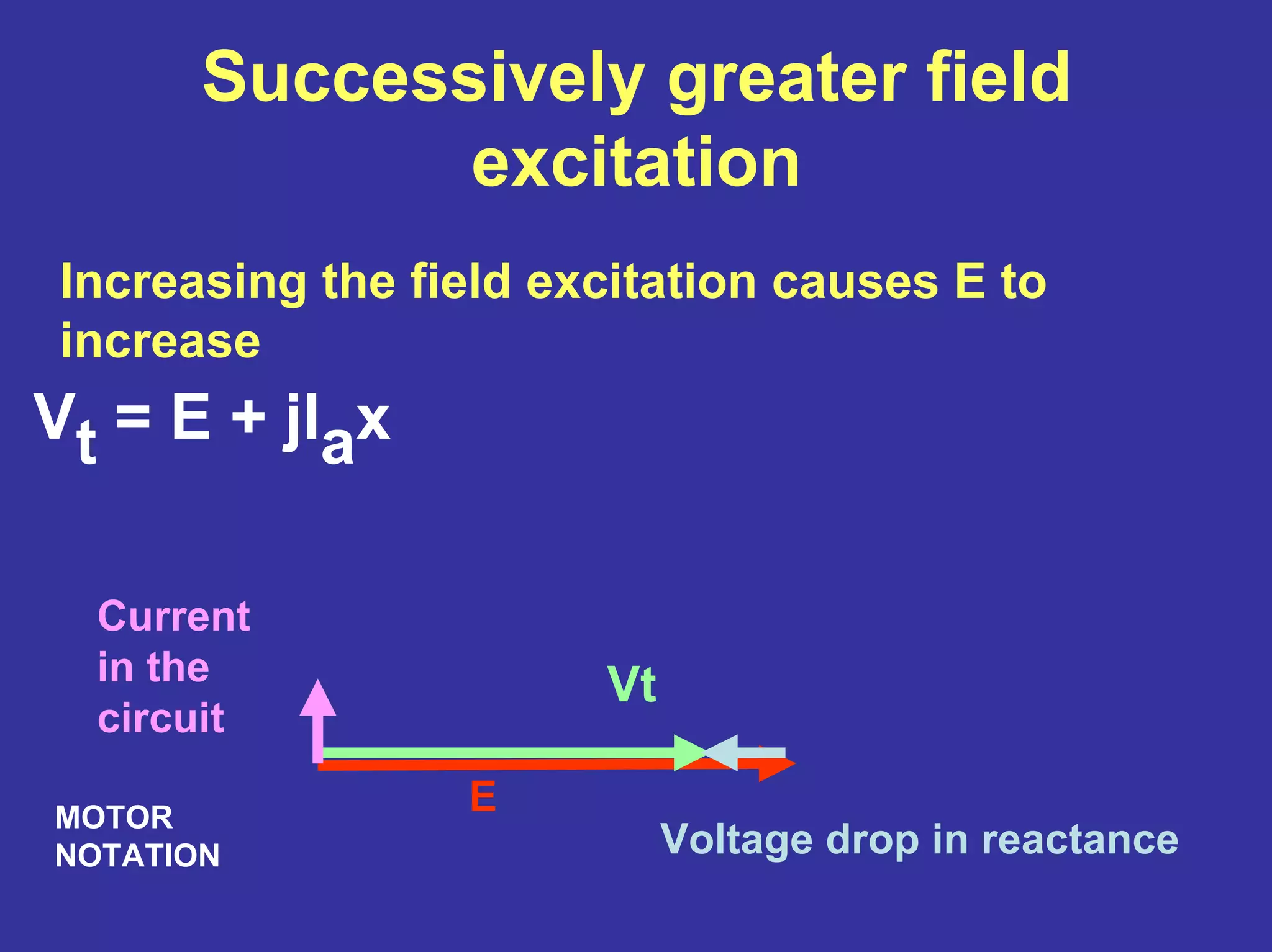
The foregoing indicatesthat as the machine
(1) approaches zero power operation – the
borderline between generator and motor
operation, the active power to/from the
machine goes to zero and (2) as the machine
becomes overexcited, the power factor
becomes cos(90) = 0.
As the field excitation increases, |E|
increases, and the machine current becomes
higher – but the power factor is still zero.
And I leads Vt. In theory, there is no active
power transferred, but a high and
controllable level of Q.
This mode of operation is called a
synchronous condenser
Synchronous condenser
operation
E
Vt
jIax
Ia
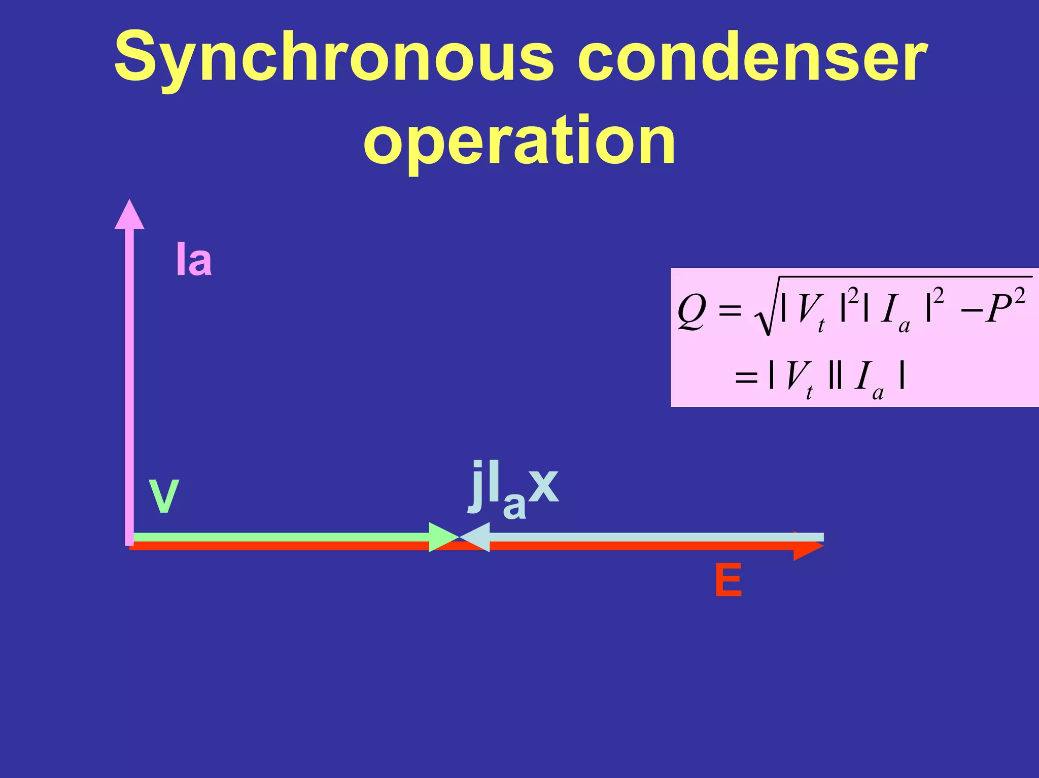
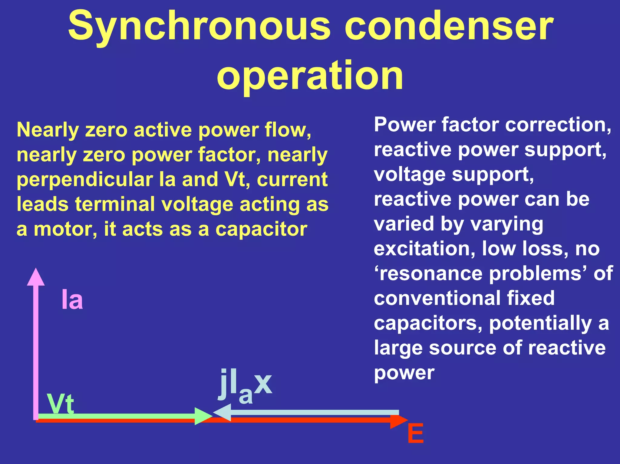
Nearly zeroactive power flow,
nearly zero power factor, nearly
perpendicular Ia and Vt, current
leads terminal voltage acting as
a motor, it acts as a capacitor
Power factor correction,
reactive power support,
voltage support,
reactive power can be
varied by varying
excitation, low loss, no
‘resonance problems’ of
conventional fixed
capacitors, potentially a
large source of reactive
power
38.
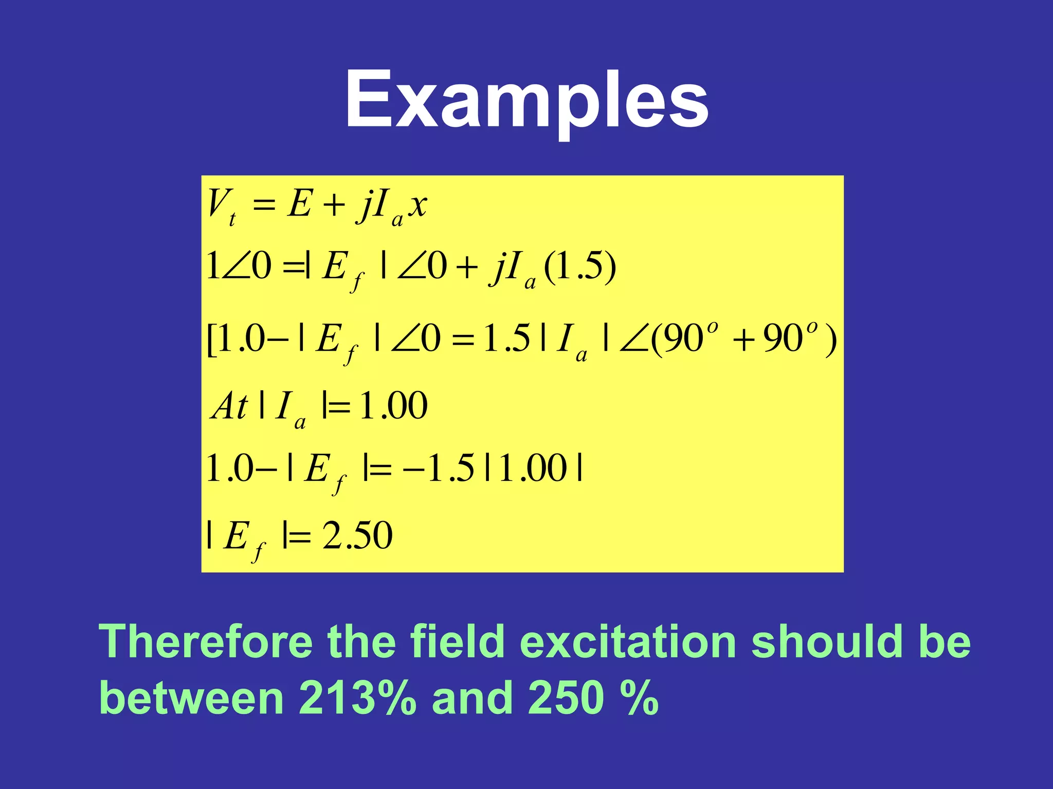
Examples
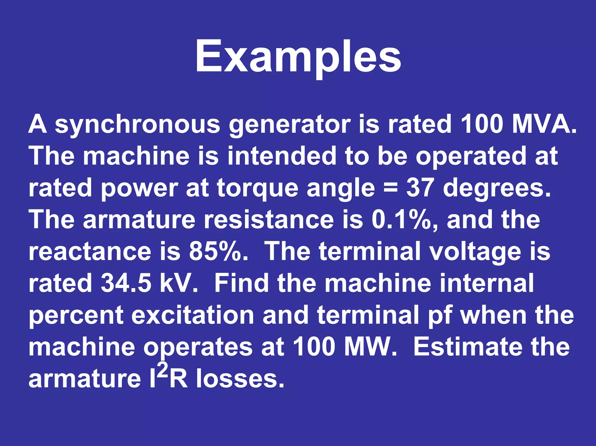
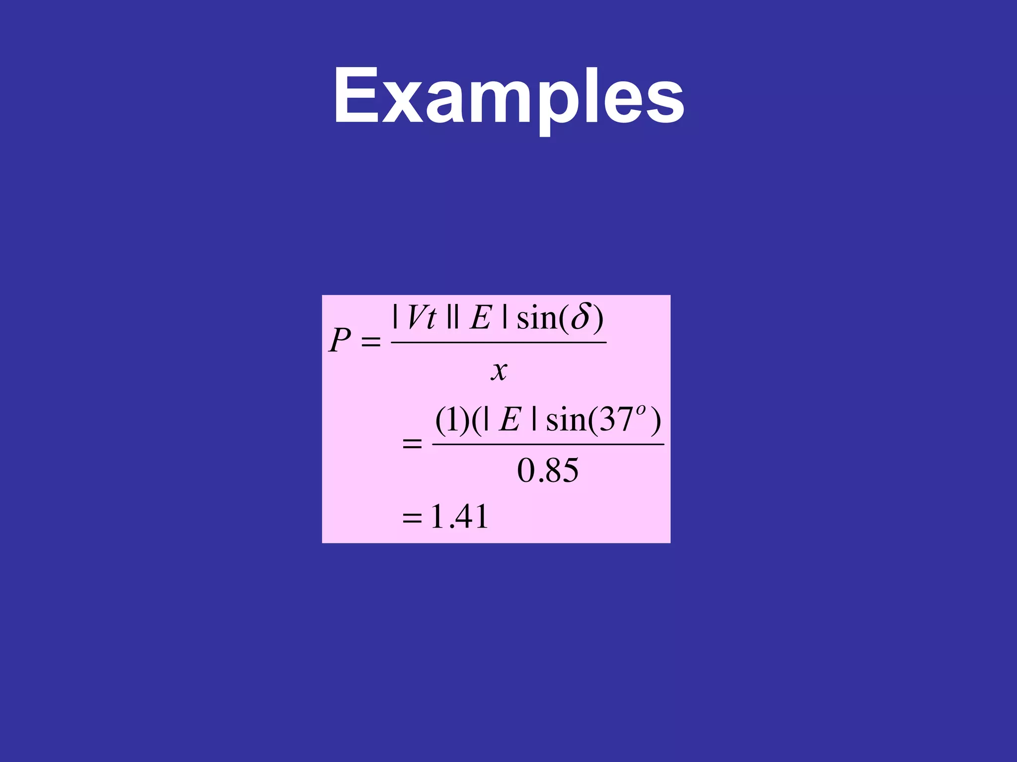
A synchronous generatoris rated 100 MVA.
The machine is intended to be operated at
rated power at torque angle = 37 degrees.
The armature resistance is 0.1%, and the
reactance is 85%. The terminal voltage is
rated 34.5 kV. Find the machine internal
percent excitation and terminal pf when the
machine operates at 100 MW. Estimate the
armature I2R losses.
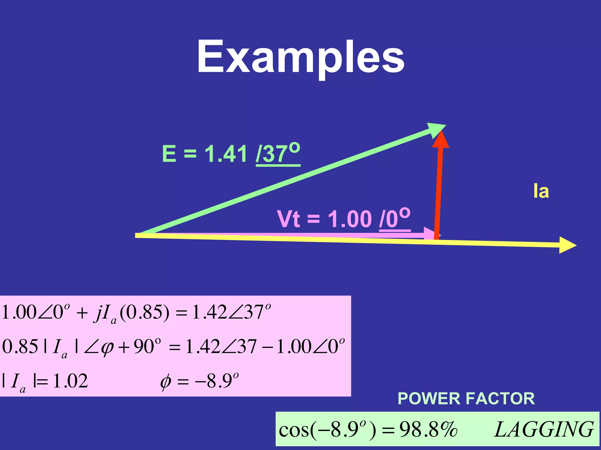
Examples
E = 1.41/37o
Vt = 1.00 /0o
o
a
o
a
o
a
o
I
I
jI
9.802.1||
000.13742.190||85.0
3742.1)85.0(000.1
o
−==
∠−∠=+∠
∠=+∠
φ
ϕ
LAGGINGo
%8.98)9.8cos( =−
POWER FACTOR
Ia
41.
Examples
A six polesynchronous generator
operates at 60 Hz. Find the speed of
operation
Examples
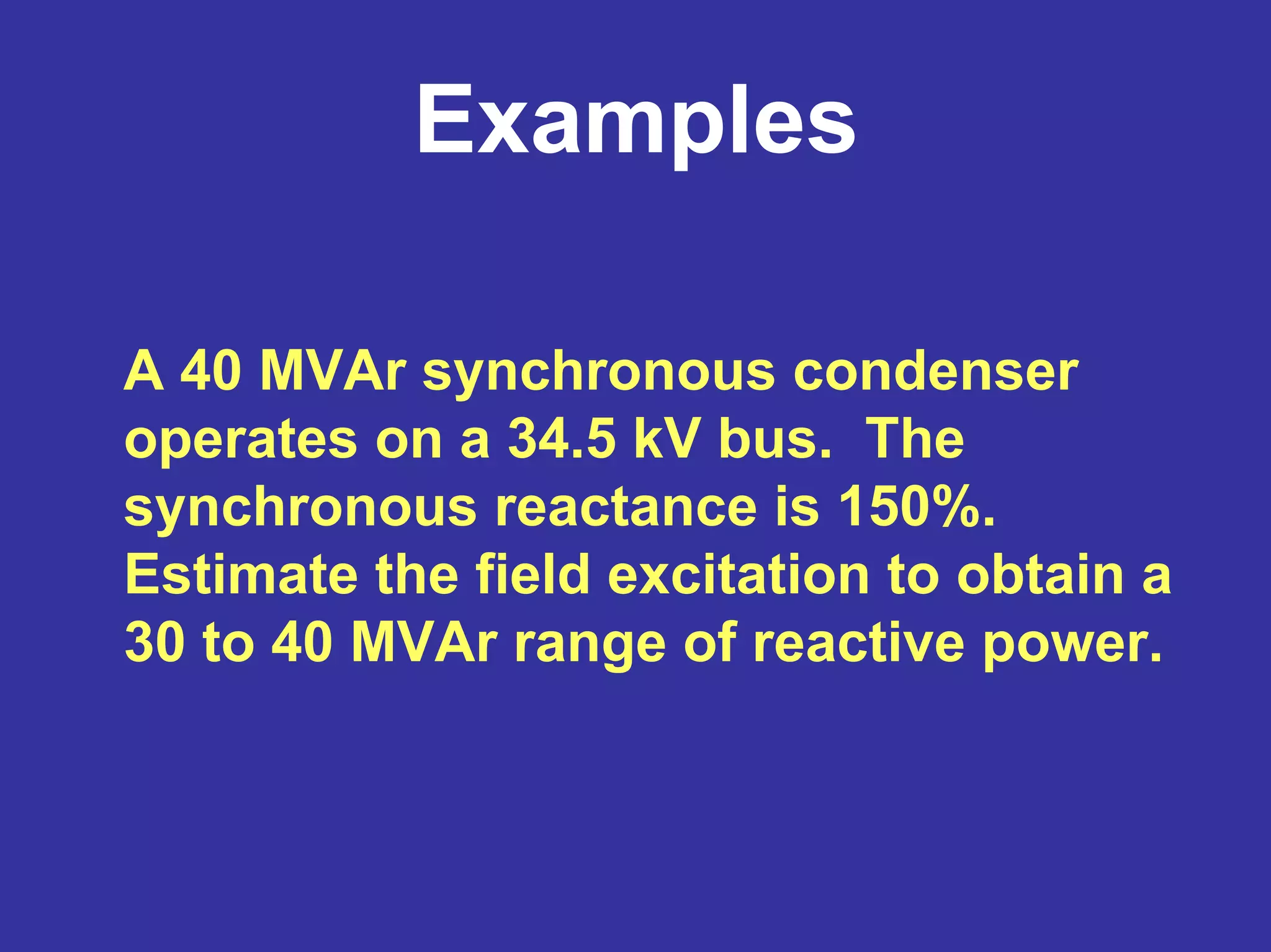
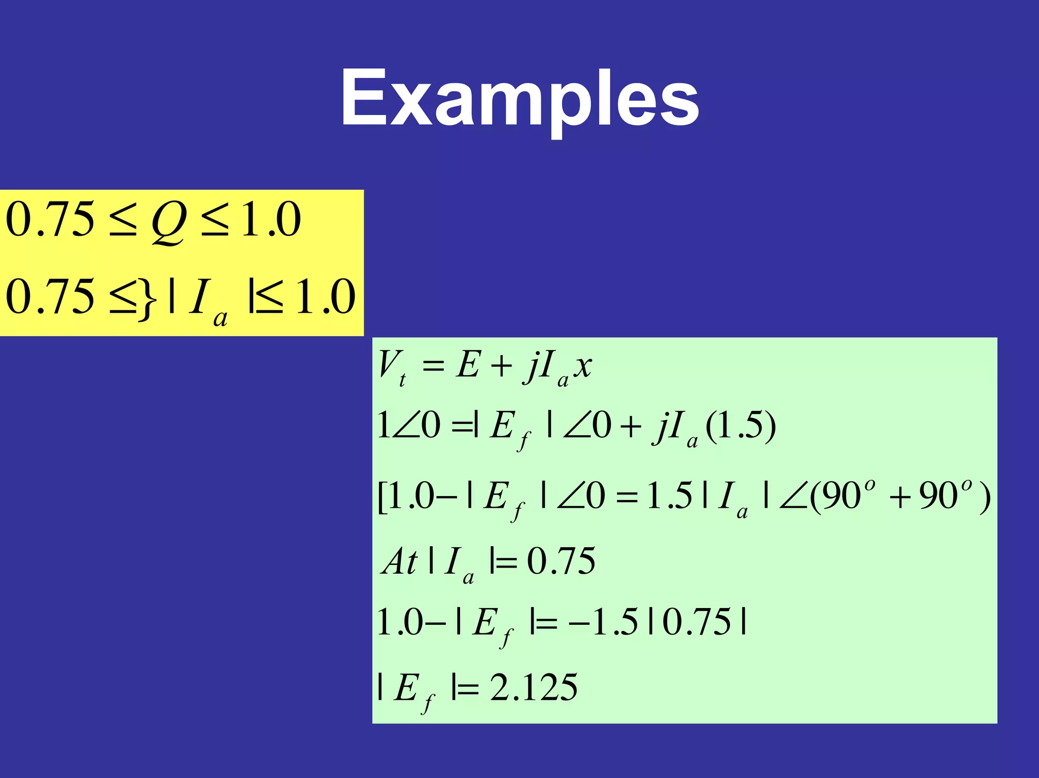
A 40 MVArsynchronous condenser
operates on a 34.5 kV bus. The
synchronous reactance is 150%.
Estimate the field excitation to obtain a
30 to 40 MVAr range of reactive power.
• Saturation andthe
magnetization curve
• Park’s transformation
• Transient and subtransient
reactances, formulas for
calculation
• Machine transients
48.
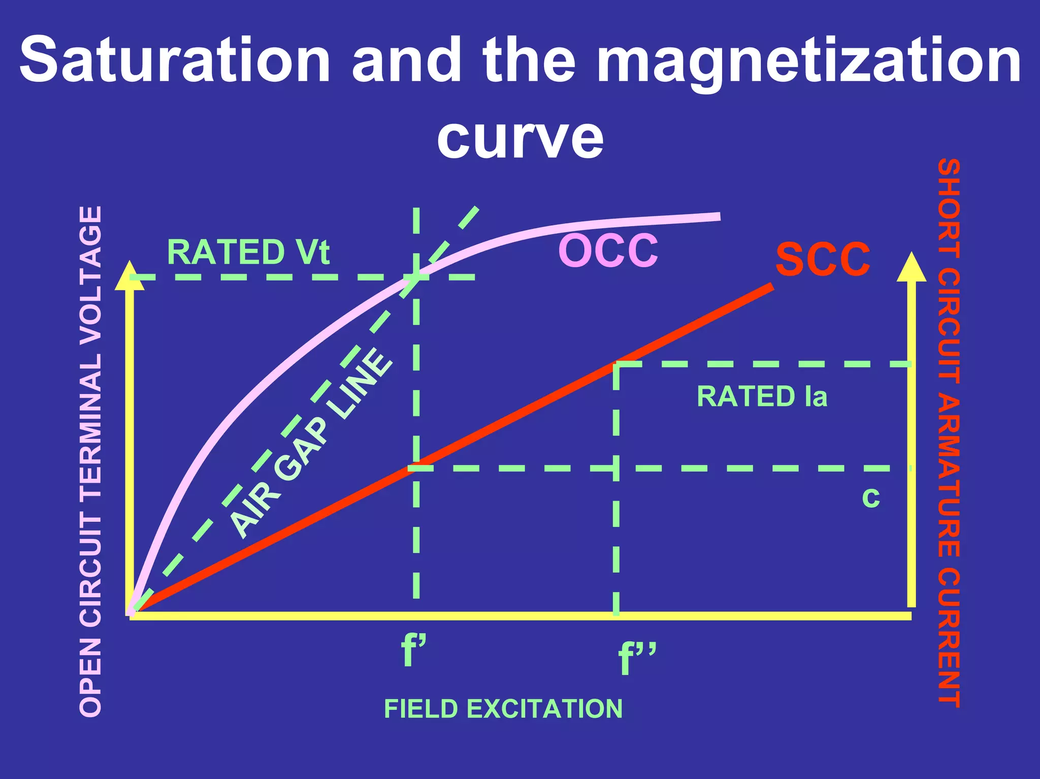
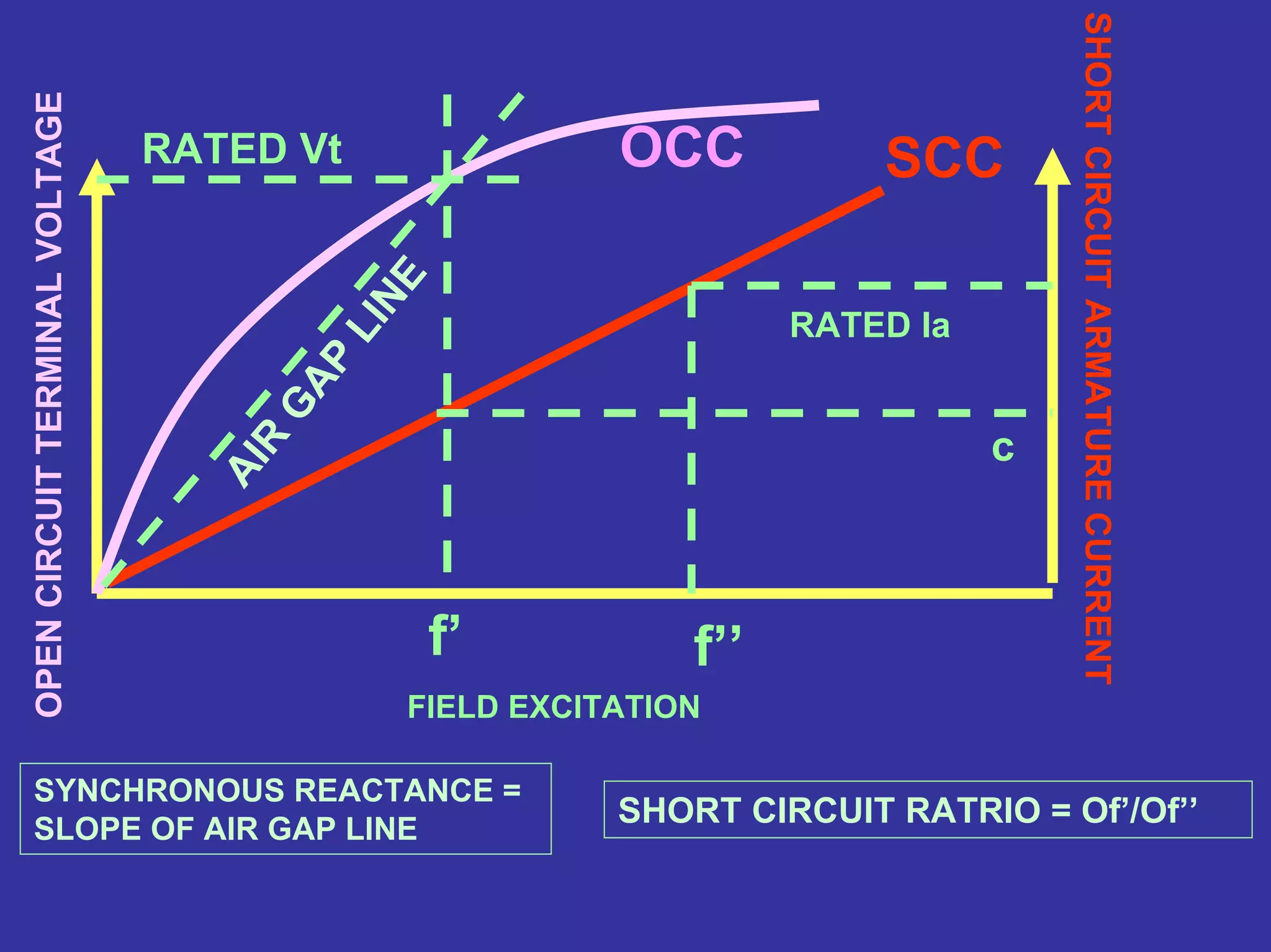
Saturation and themagnetization
curve
FIELD EXCITATION
SHORTCIRCUITARMATURECURRENT
OPENCIRCUITTERMINALVOLTAGE
RATED Ia
SCC
c
f’’f’
RATED Vt OCC
AIR
G
AP
LINE
Saturation and themagnetization
curve
• Saturation occurs because of the alignment
of magnetic domains. When most of the
domains align, the material saturates and no
little further magnetization can occur
• Saturation is mainly a property of iron -- it
does not manifest itself over a practical
range of fluxes in air, plastic, or other non-
ferrous materials
• The effect of saturation is to lower the
synchronous reactance (to a ‘saturated
value’)
51.
Saturation and themagnetization
curve
• Saturation may limit the performance of
machines because of high air gap line
voltage drop
• Saturation is often accompanied by
hysteresis which results in losses in
AC machines
• Saturation is not present in
superconducting machines
52.
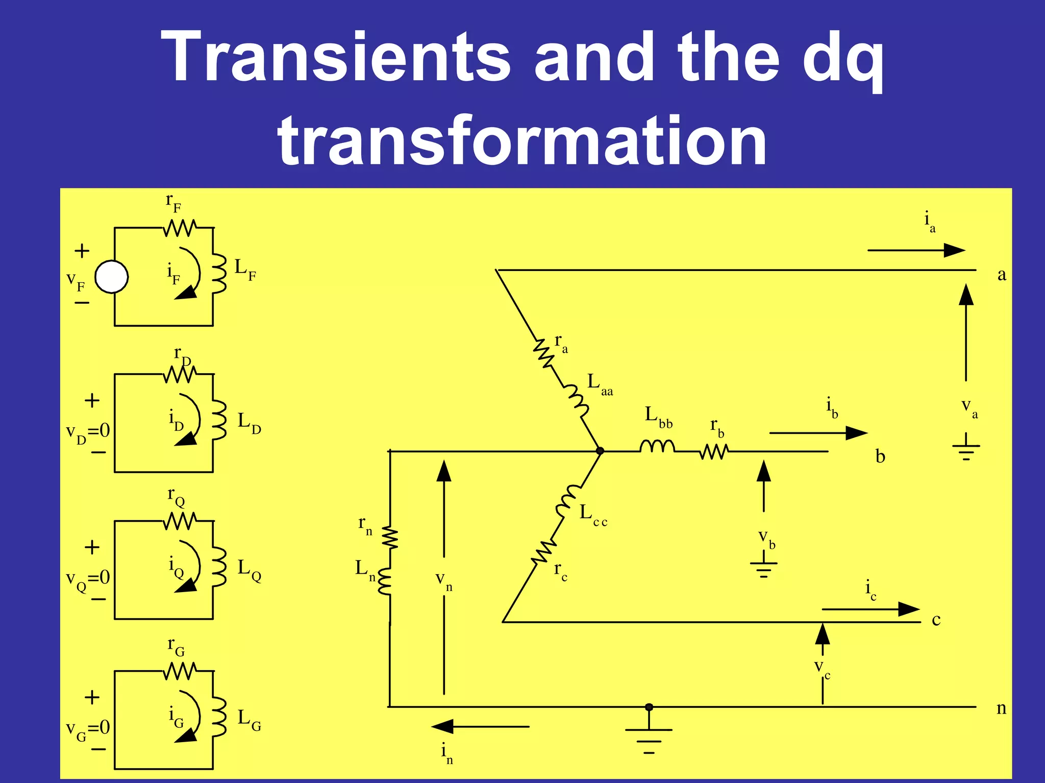
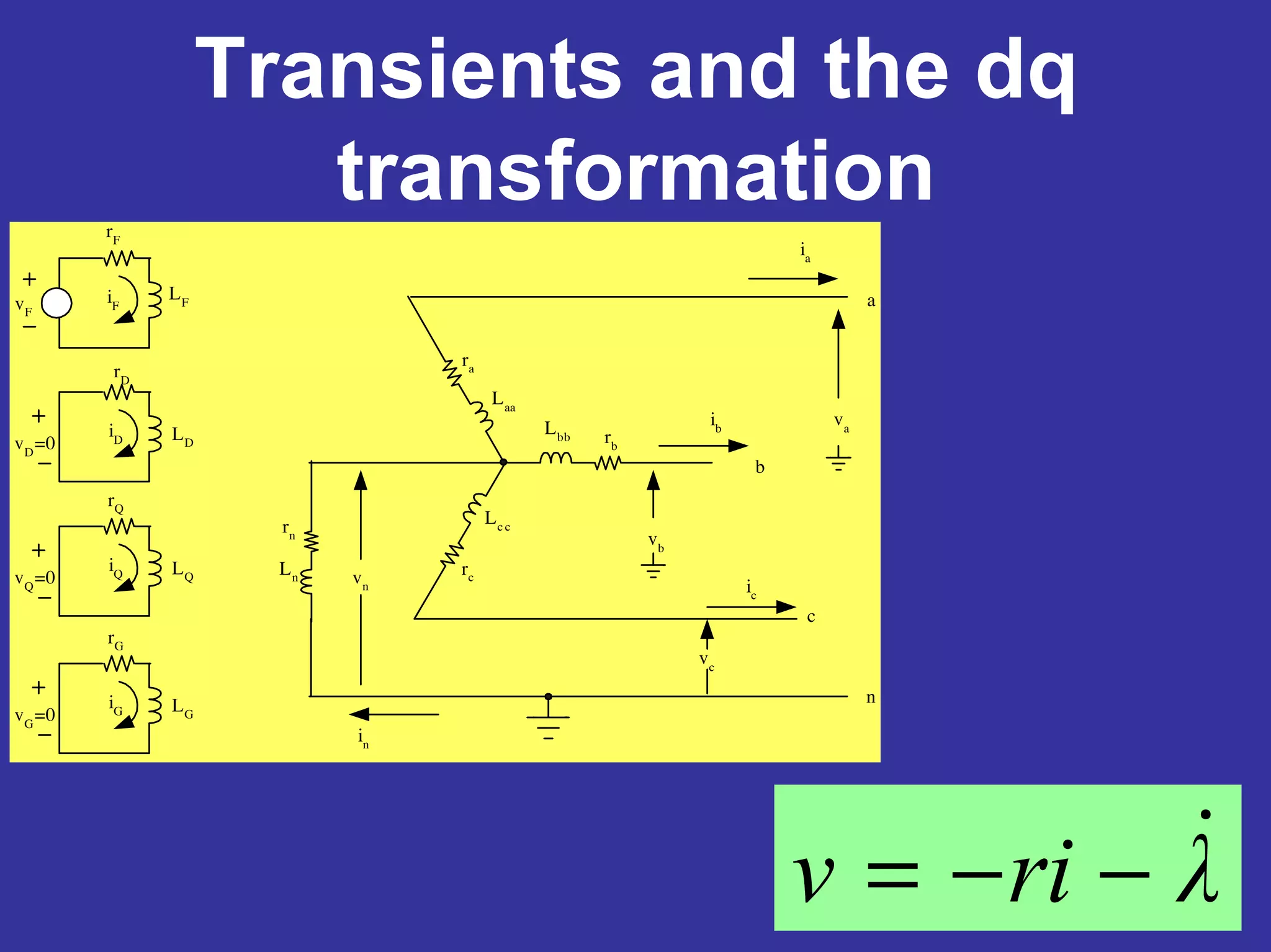
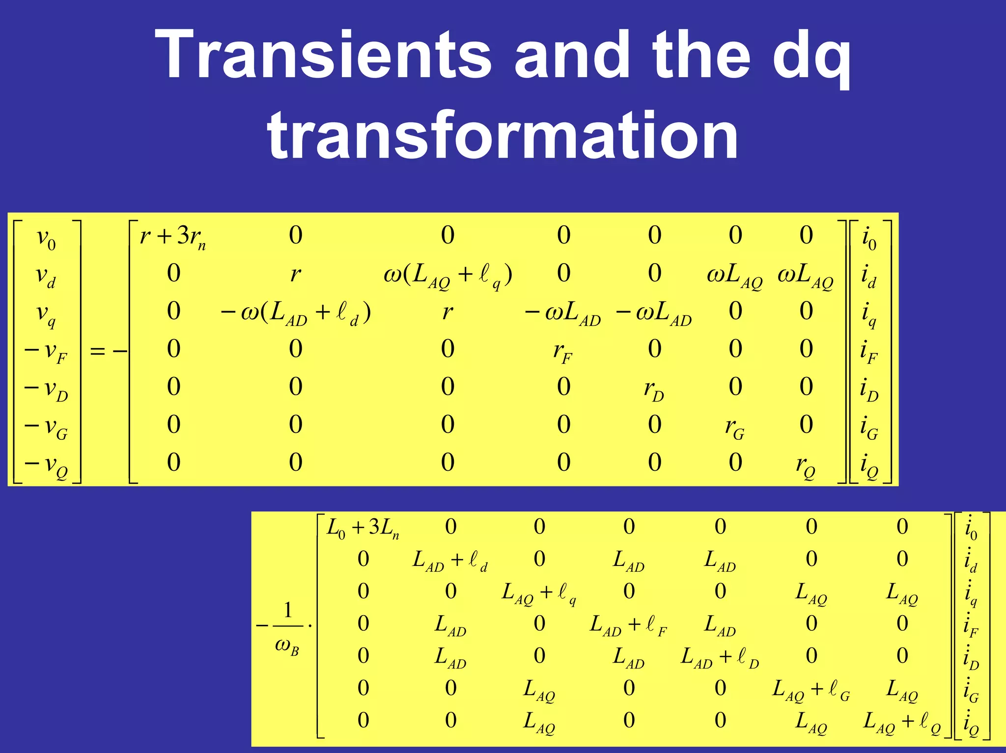
Transients and thedq
transformation
Lbb
rc
ra
rb
rn
Laa
Lc c
Ln
va
vb
vn ic
ib
ia
in
a
b
c
n
vc
rD
LDvD
=0
iD
rG
LGvG
=0
iG
rF
LFiFvF
rQ
LQvQ
=0
iQ
53.
Transients and thedq
transformation
Lbb
rc
ra
rb
rn
Laa
Lc c
Ln
va
vb
vn ic
ib
ia
in
a
b
c
n
vc
rD
LDvD
=0
iD
rG
LGvG
=0
iG
rF
LFiFvF
rQ
LQvQ
=0
iQ
λriv −−=
54.
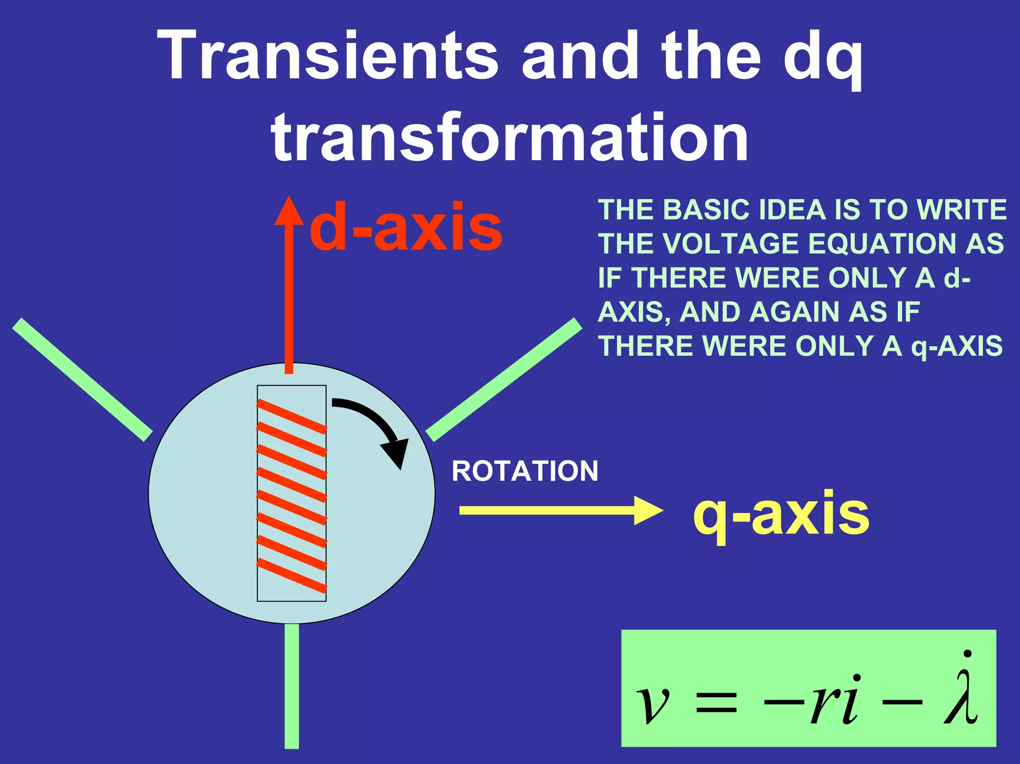
Transients and thedq
transformation
λriv −−=
ROTATION
d-axis
q-axis
THE BASIC IDEA IS TO WRITE
THE VOLTAGE EQUATION AS
IF THERE WERE ONLY A d-
AXIS, AND AGAIN AS IF
THERE WERE ONLY A q-AXIS
55.
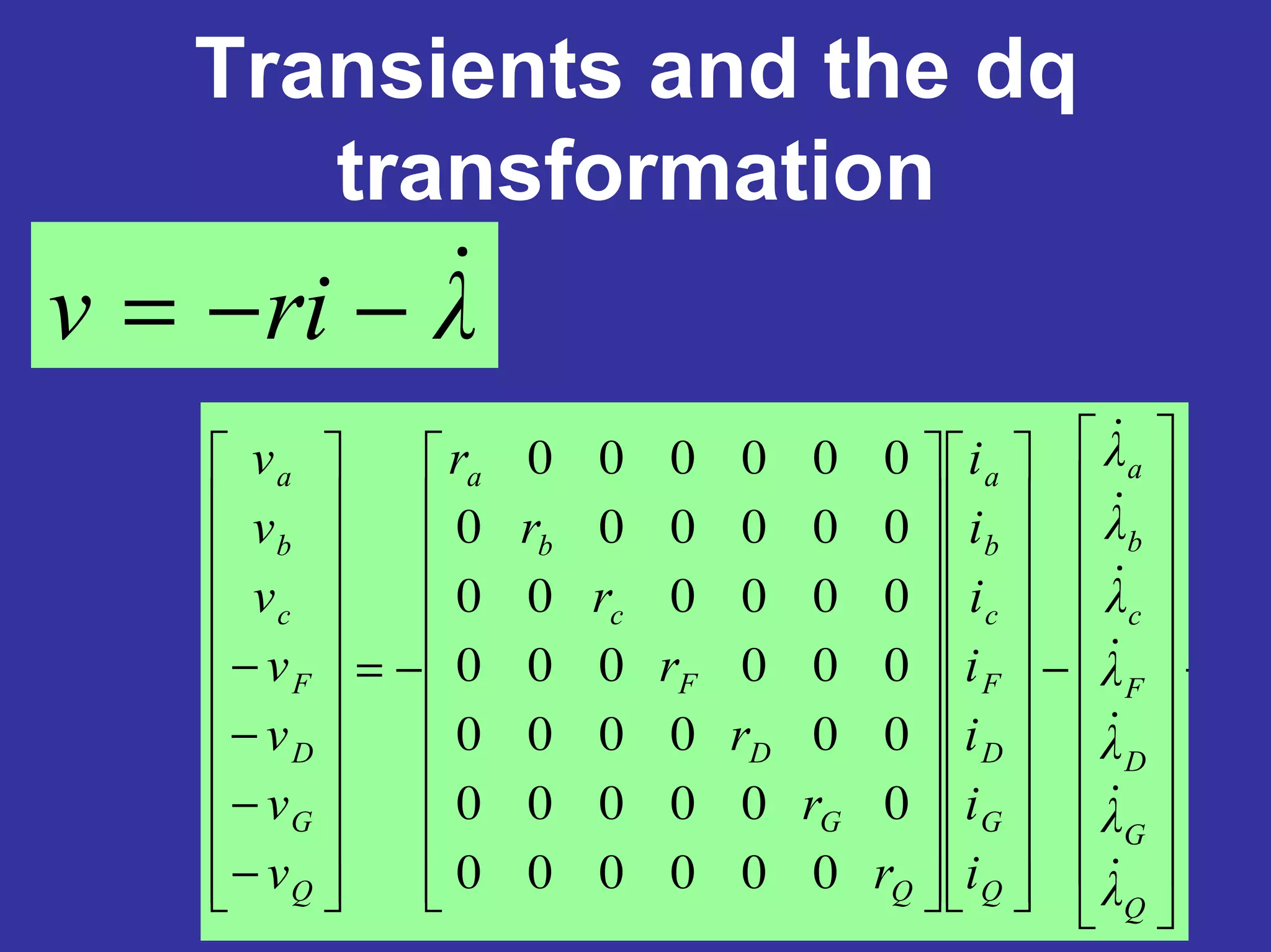
Transients and thedq
transformation
λriv −−=
+−−=
−
−
−
−
000000
000000
000000
000000
000000
000000
000000
Q
G
D
F
c
b
a
Q
G
D
F
c
b
a
Q
G
D
F
c
b
a
Q
G
D
F
c
b
a
λ
λ
λ
λ
λ
λ
λ
i
i
i
i
i
i
i
r
r
r
r
r
r
r
v
v
v
v
v
v
v
56.
Transients and thedq
transformation
+−
+−=
)
3
2sin()
3
2sin(sin
)
3
2cos()
3
2cos(cos
2
1
2
1
2
1
3
2P
πθπθθ
πθπθθ
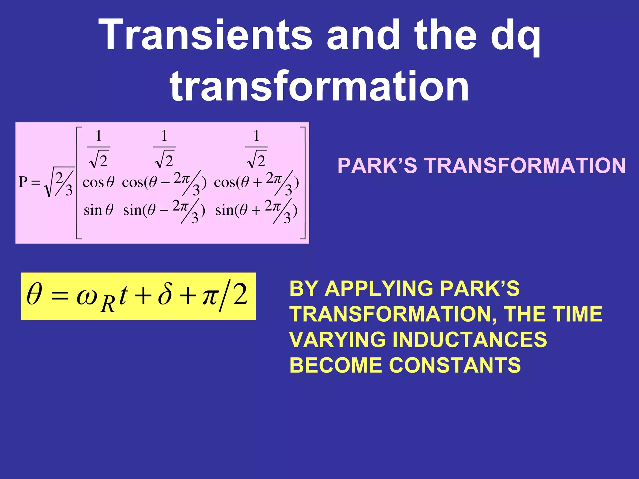
PARK’S TRANSFORMATION
2πδtωθ R ++= BY APPLYING PARK’S
TRANSFORMATION, THE TIME
VARYING INDUCTANCES
BECOME CONSTANTS
57.
Transients and thedq
transformation
−−+−
+
+
−=
−
−
−
−
Q
G
D
F
q
d
Q
G
D
F
ADADdAD
AQAQqAQ
n
Q
G
D
F
q
d
i
i
i
i
i
i
i
r
r
r
r
LωLωrLω
LωLωLωr
rr
v
v
v
v
v
v
v 00
000000
000000
000000
000000
00)(0
00)(0
0000003
+
+
+
+
+
+
+
⋅−
Q
G
D
F
q
d
QAQAQAQ
AQGAQAQ
DADADAD
ADFADAD
AQAQqAQ
ADADdAD
n
B
i
i
i
i
i
i
i
LLL
LLL
LLL
LLL
LLL
LLL
LL
ω
00
0000
0000
0000
0000
0000
0000
0000003
1
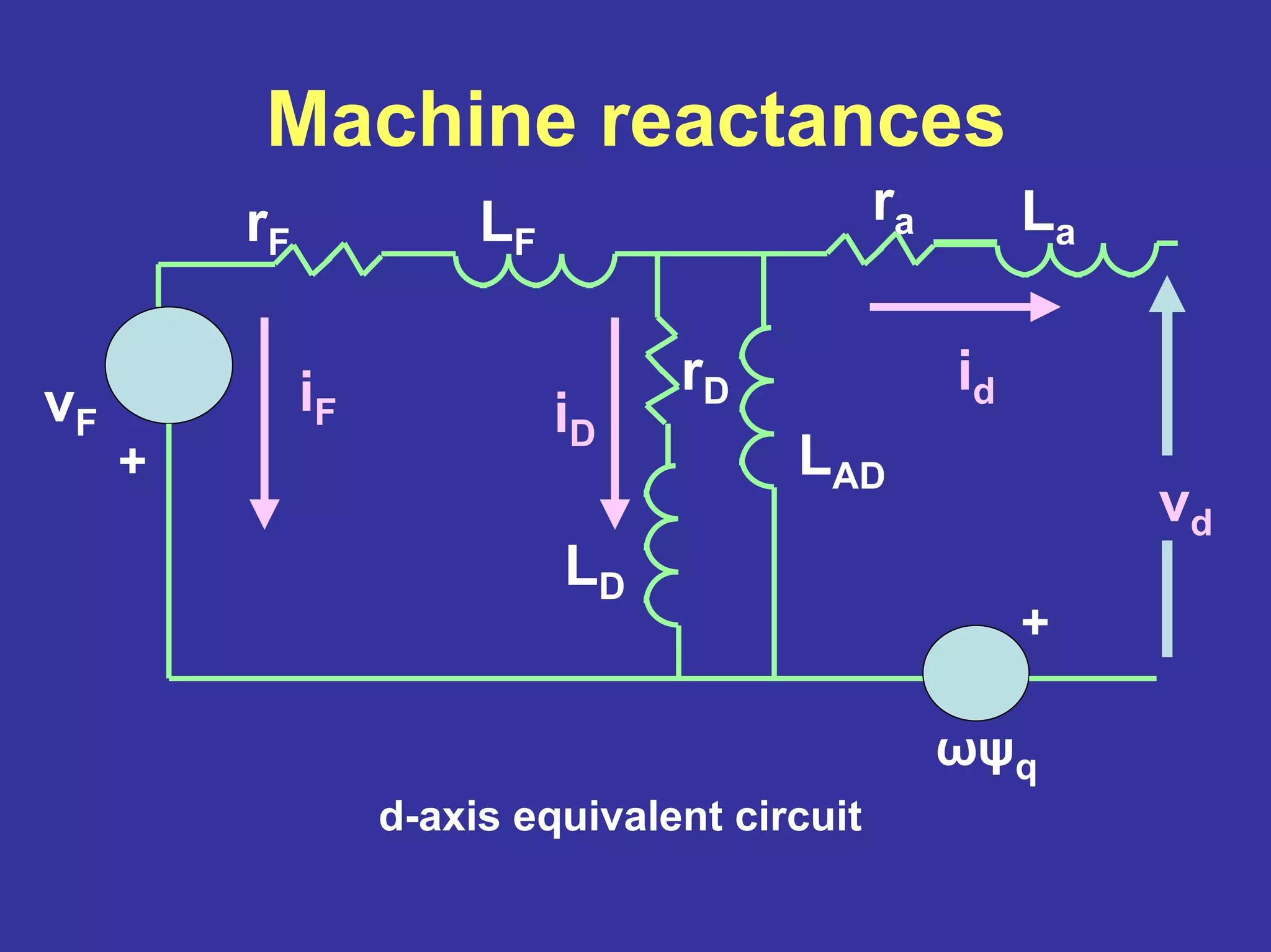
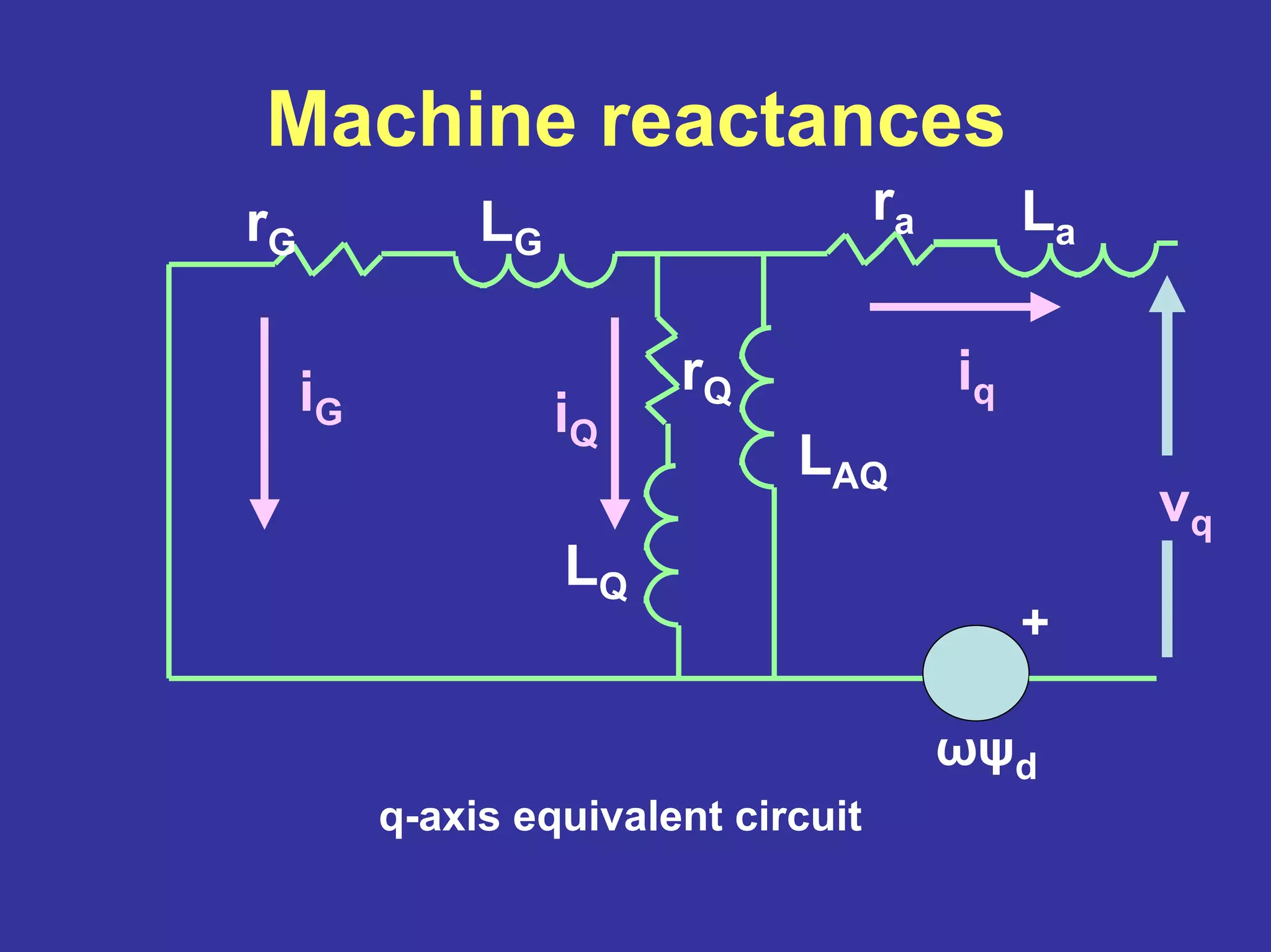
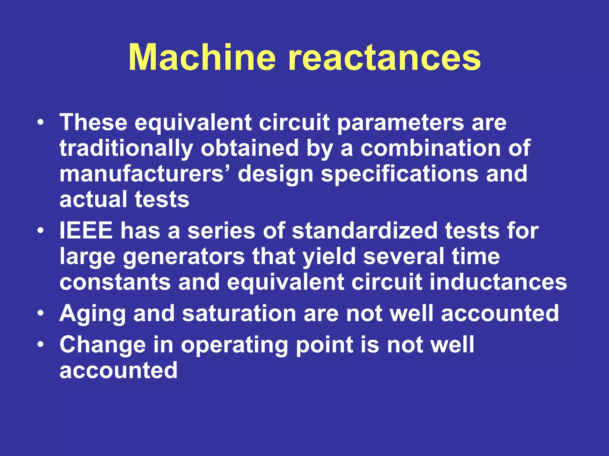
Machine reactances
• Theseequivalent circuit parameters are
traditionally obtained by a combination of
manufacturers’ design specifications and
actual tests
• IEEE has a series of standardized tests for
large generators that yield several time
constants and equivalent circuit inductances
• Aging and saturation are not well accounted
• Change in operating point is not well
accounted
61.
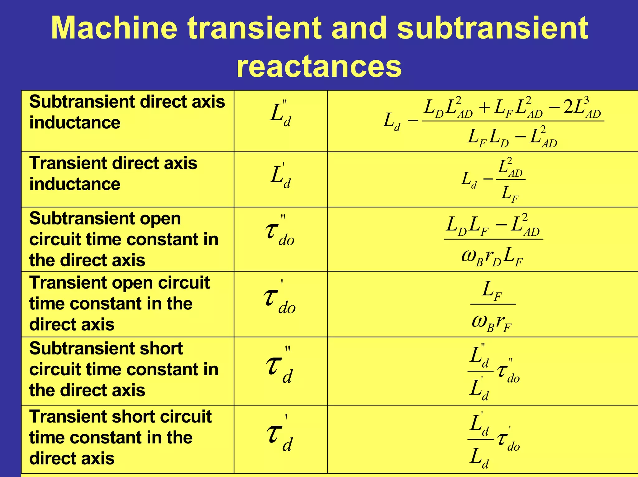
Machine transient andsubtransient
reactances
Subtransient direct axis
inductance
"
dL
2
322
2
ADDF
ADADFADD
d
LLL
LLLLL
L
−
−+
−
Transient direct axis
inductance
'
dL
F
AD
d
L
L
L
2
−
Subtransient open
circuit time constant in
the direct axis
"
doτ
FDB
ADFD
Lr
LLL
ω
2
−
Transient open circuit
time constant in the
direct axis
'
doτ
FB
F
r
L
ω
Subtransient short
circuit time constant in
the direct axis
"
dτ "
'
"
do
d
d
L
L
τ
Transient short circuit
time constant in the
direct axis
'
dτ '
'
do
d
d
L
L
τ
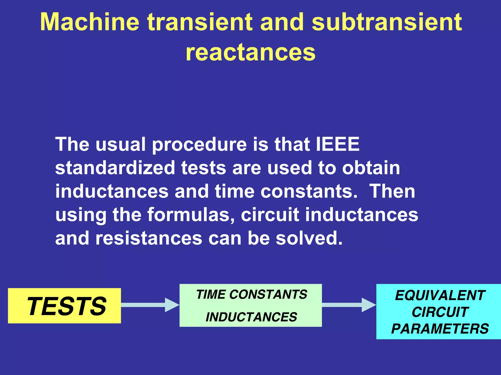
Machine transient andsubtransient
reactances
The usual procedure is that IEEE
standardized tests are used to obtain
inductances and time constants. Then
using the formulas, circuit inductances
and resistances can be solved.
TESTS
TIME CONSTANTS
INDUCTANCES
EQUIVALENT
CIRCUIT
PARAMETERS
66.
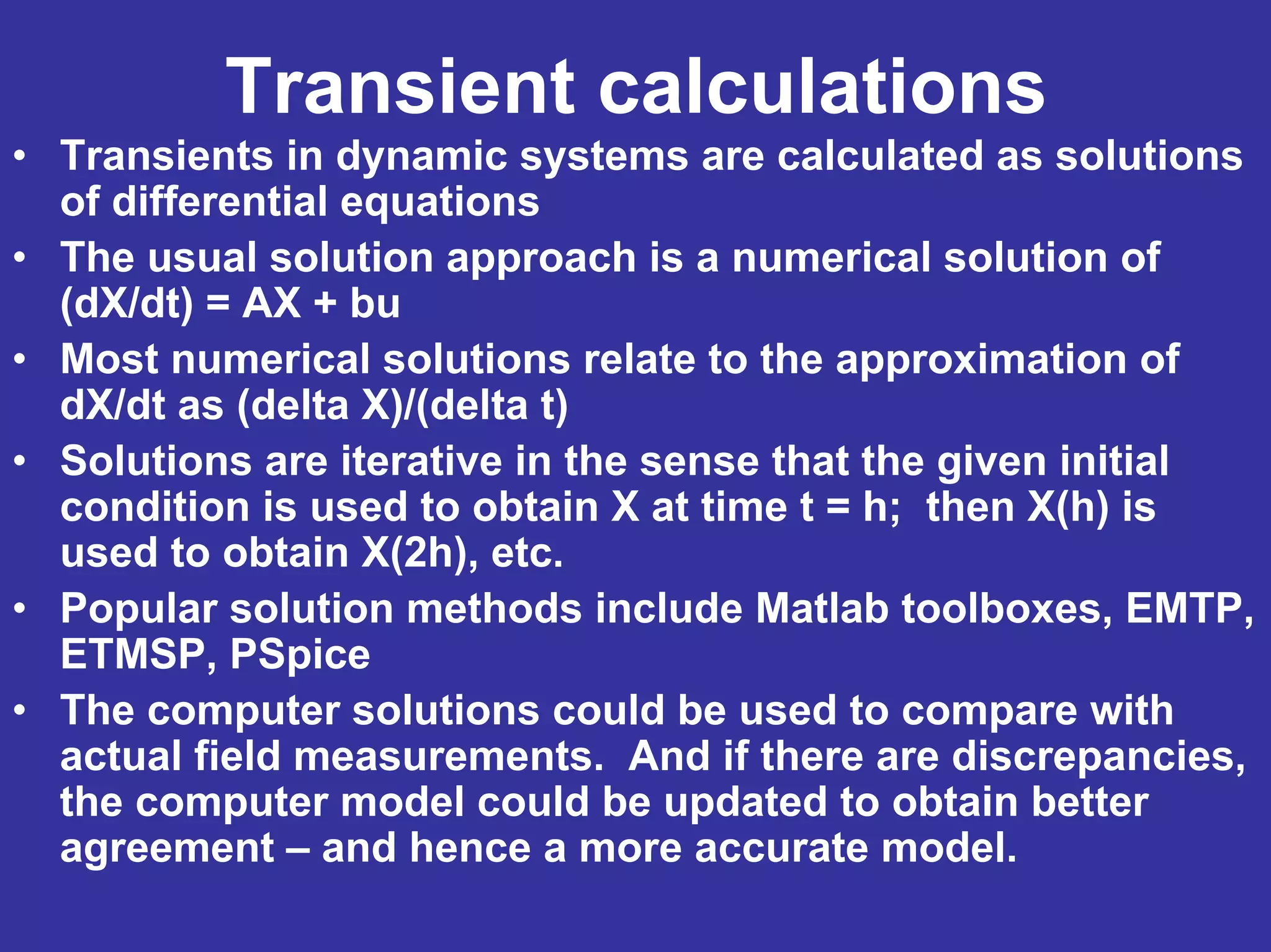
Transient calculations
• Transientsin dynamic systems are calculated as solutions
of differential equations
• The usual solution approach is a numerical solution of
(dX/dt) = AX + bu
• Most numerical solutions relate to the approximation of
dX/dt as (delta X)/(delta t)
• Solutions are iterative in the sense that the given initial
condition is used to obtain X at time t = h; then X(h) is
used to obtain X(2h), etc.
• Popular solution methods include Matlab toolboxes, EMTP,
ETMSP, PSpice
• The computer solutions could be used to compare with
actual field measurements. And if there are discrepancies,
the computer model could be updated to obtain better
agreement – and hence a more accurate model.
• Basics ofstate estimation
• Application to synchronous generators
• Demonstration of software to identify
synchronous generator parameters
Session topics:
69.
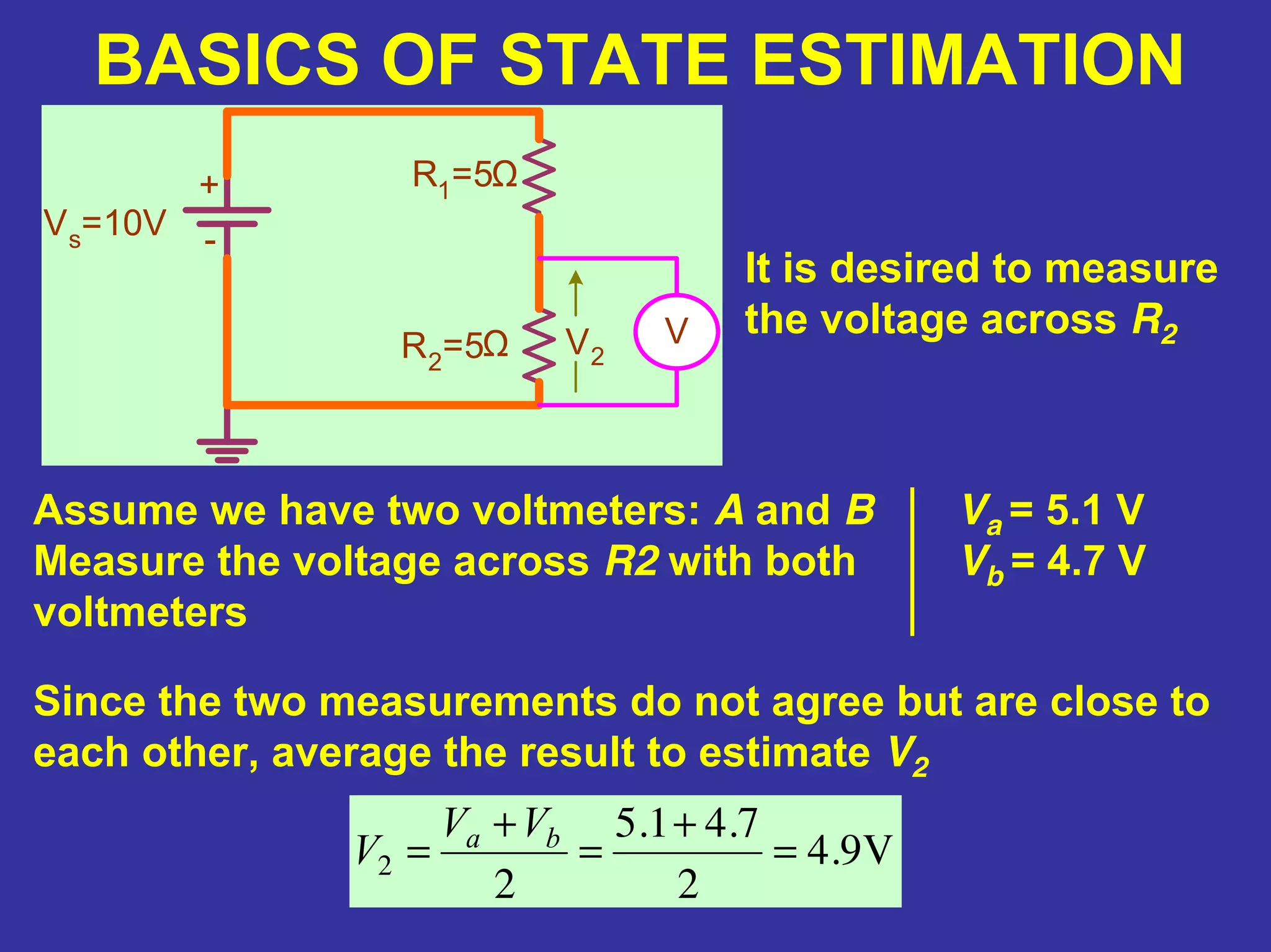
BASICS OF STATEESTIMATION
It is desired to measure
the voltage across R2
Va = 5.1 V
Vb = 4.7 V
Since the two measurements do not agree but are close to
each other, average the result to estimate V2
V9.4
2
7.41.5
2
2 =
+
=
+
= ba VV
V
Vs=10V
R1
=5
R2=5 VV2
Ω
Ω
-
+
Assume we have two voltmeters: A and B
Measure the voltage across R2 with both
voltmeters
70.
BASICS OF STATEESTIMATION
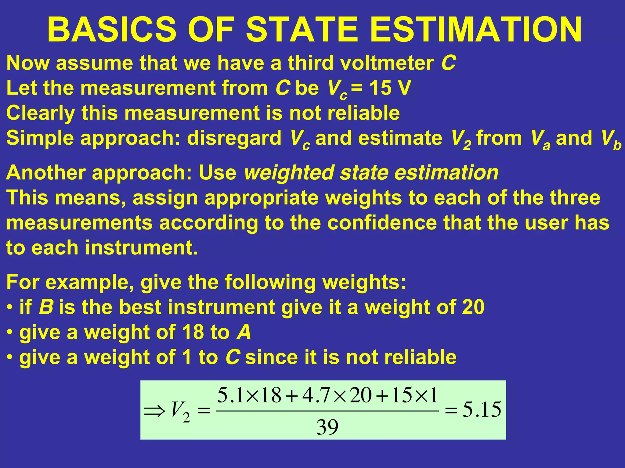
Now assume that we have a third voltmeter C
Let the measurement from C be Vc = 15 V
Clearly this measurement is not reliable
Simple approach: disregard Vc and estimate V2 from Va and Vb
Another approach: Use weighted state estimation
This means, assign appropriate weights to each of the three
measurements according to the confidence that the user has
to each instrument.
For example, give the following weights:
• if B is the best instrument give it a weight of 20
• give a weight of 18 to A
• give a weight of 1 to C since it is not reliable
15.5
39
115207.4181.5
2 =
×+×+×
=⇒V
71.
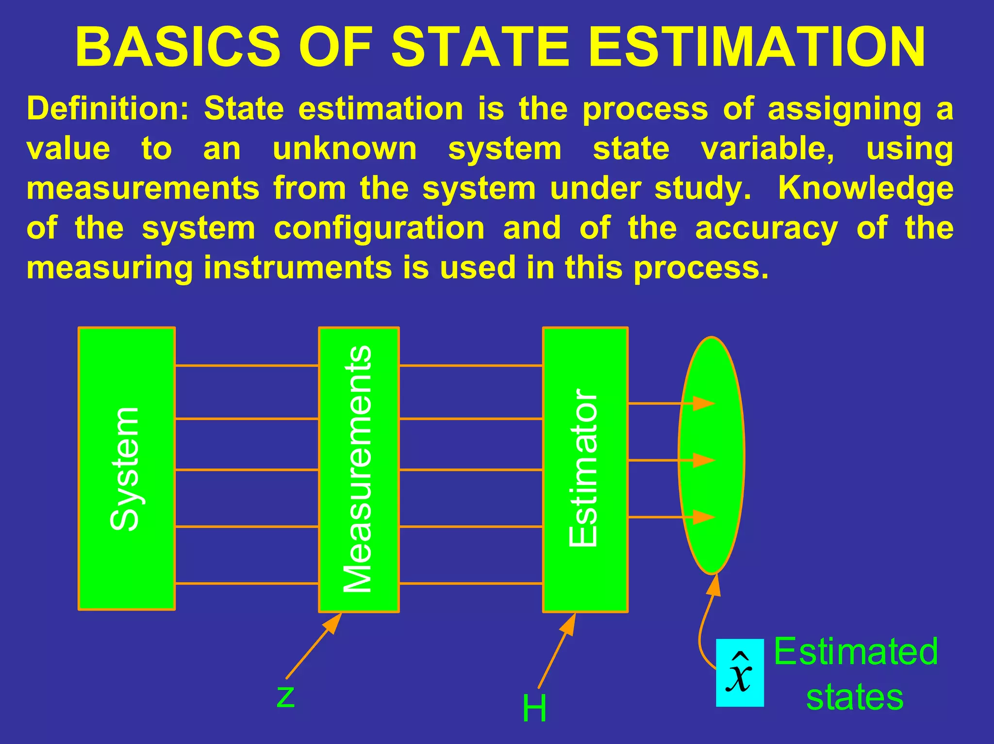
BASICS OF STATEESTIMATION
Definition: State estimation is the process of assigning a
value to an unknown system state variable, using
measurements from the system under study. Knowledge
of the system configuration and of the accuracy of the
measuring instruments is used in this process.
Estimated
states
System
Measurements
Estimator
xˆz H
72.
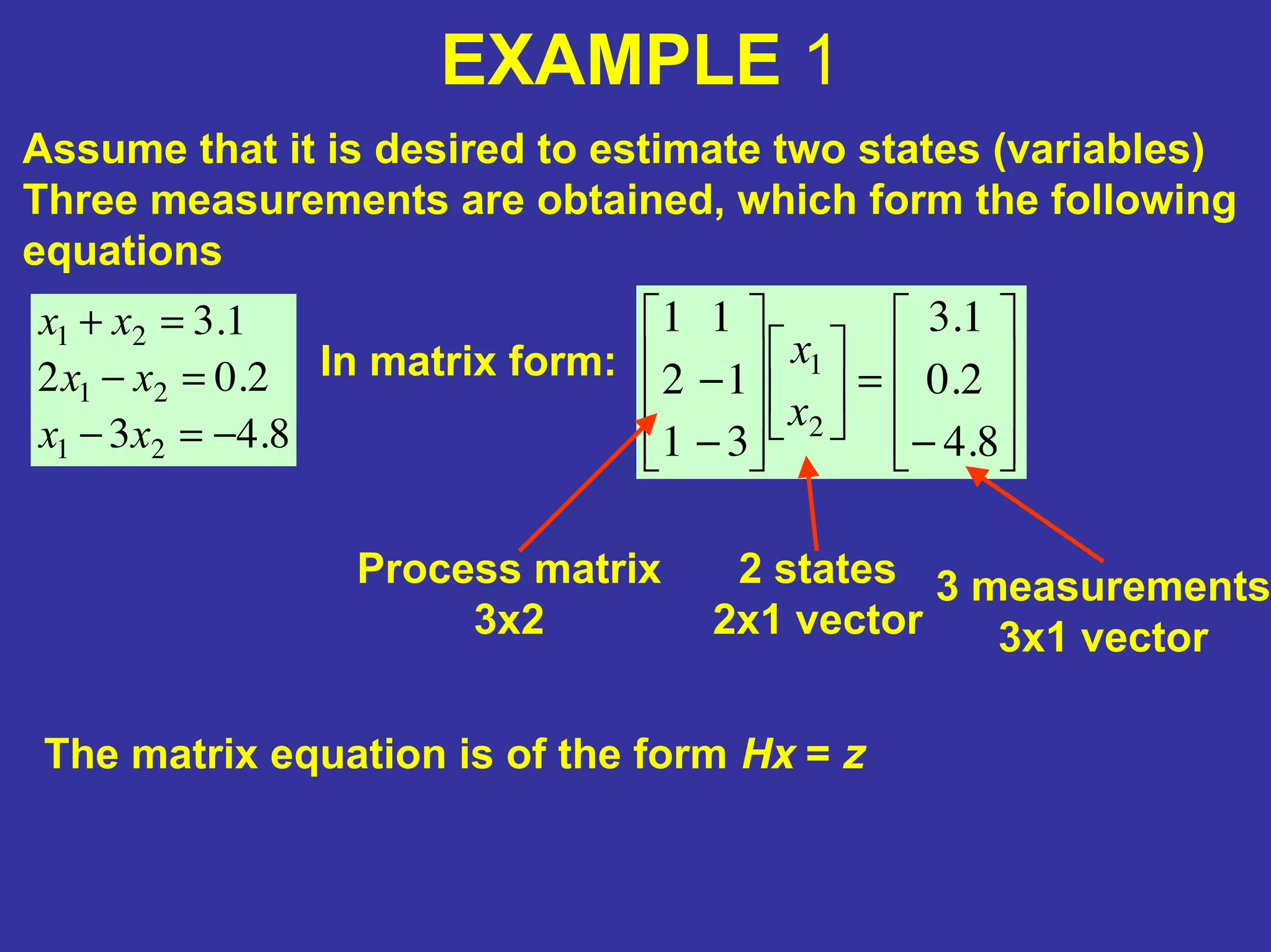
EXAMPLE 1
Assume thatit is desired to estimate two states (variables)
Three measurements are obtained, which form the following
equations
8.43
2.02
1.3
21
21
21
−=−
=−
=+
xx
xx
xx
In matrix form:
−
=
−
−
8.4
2.0
1.3
31
12
11
2
1
x
x
The matrix equation is of the form Hx = z
2 states
2x1 vector
3 measurements
3x1 vector
Process matrix
3x2
73.
−
=
−
−
8.4
2.0
1.3
31
12
11
2
1
x
x
EXAMPLE 1
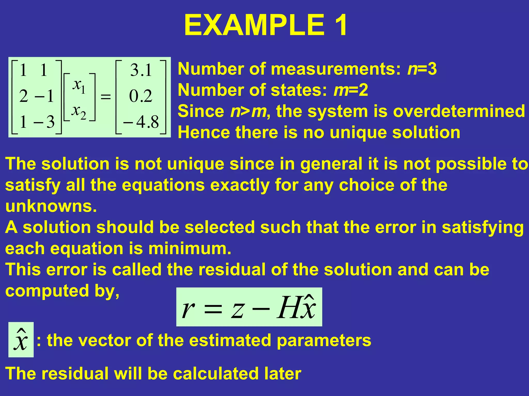
Number ofmeasurements: n=3
Number of states: m=2
Since n>m, the system is overdetermined
Hence there is no unique solution
The solution is not unique since in general it is not possible to
satisfy all the equations exactly for any choice of the
unknowns.
A solution should be selected such that the error in satisfying
each equation is minimum.
This error is called the residual of the solution and can be
computed by,
xHzr ˆ−=
xˆ : the vector of the estimated parameters
The residual will be calculated later
74.
EXAMPLE 1
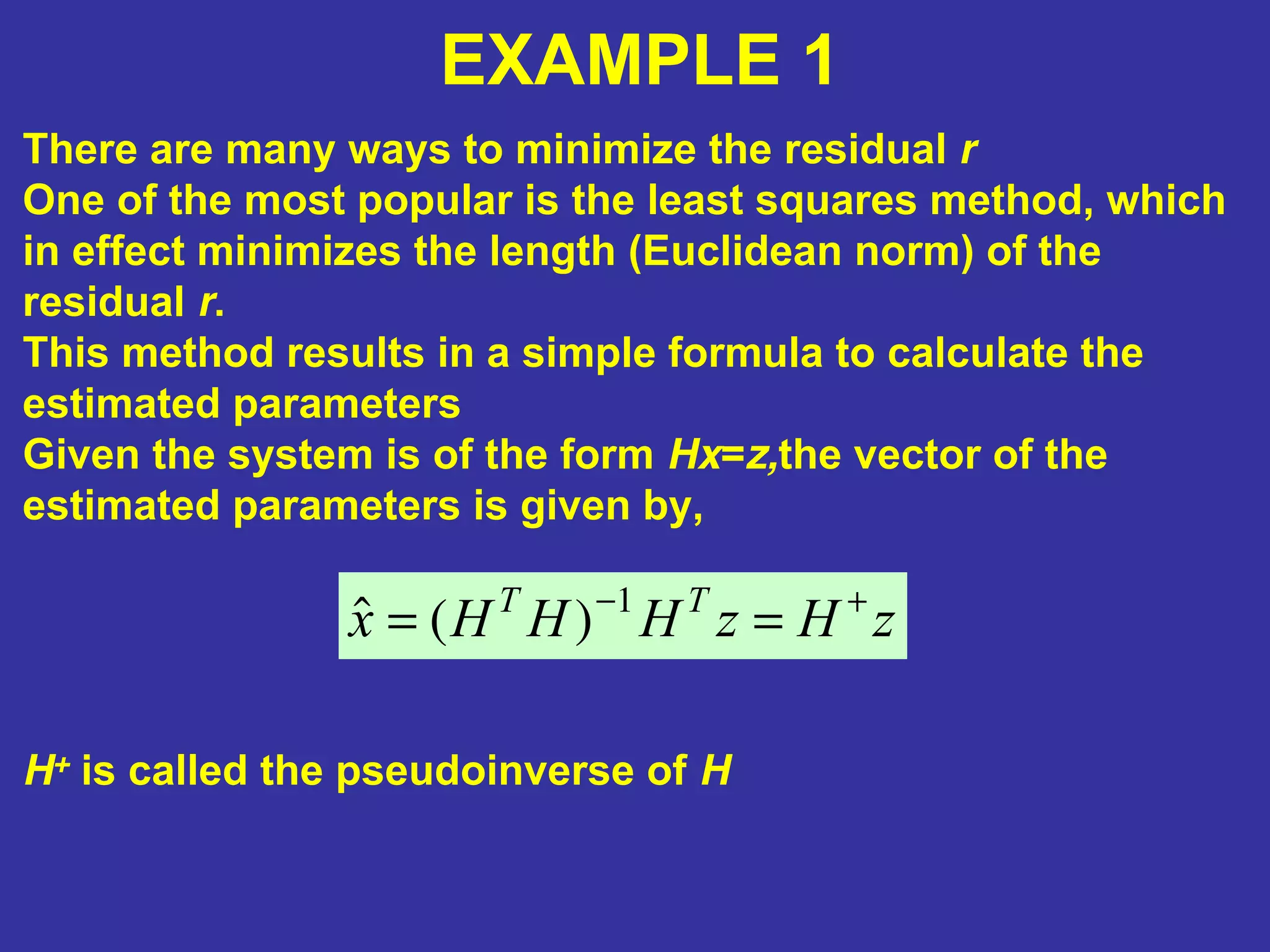
There aremany ways to minimize the residual r
One of the most popular is the least squares method, which
in effect minimizes the length (Euclidean norm) of the
residual r.
This method results in a simple formula to calculate the
estimated parameters
Given the system is of the form Hx=z,the vector of the
estimated parameters is given by,
zHzHHHx TT +−
== 1
)(ˆ
H+ is called the pseudoinverse of H
75.
−
=
−
−
8.4
2.0
1.3
31
12
11
2
1
x
x
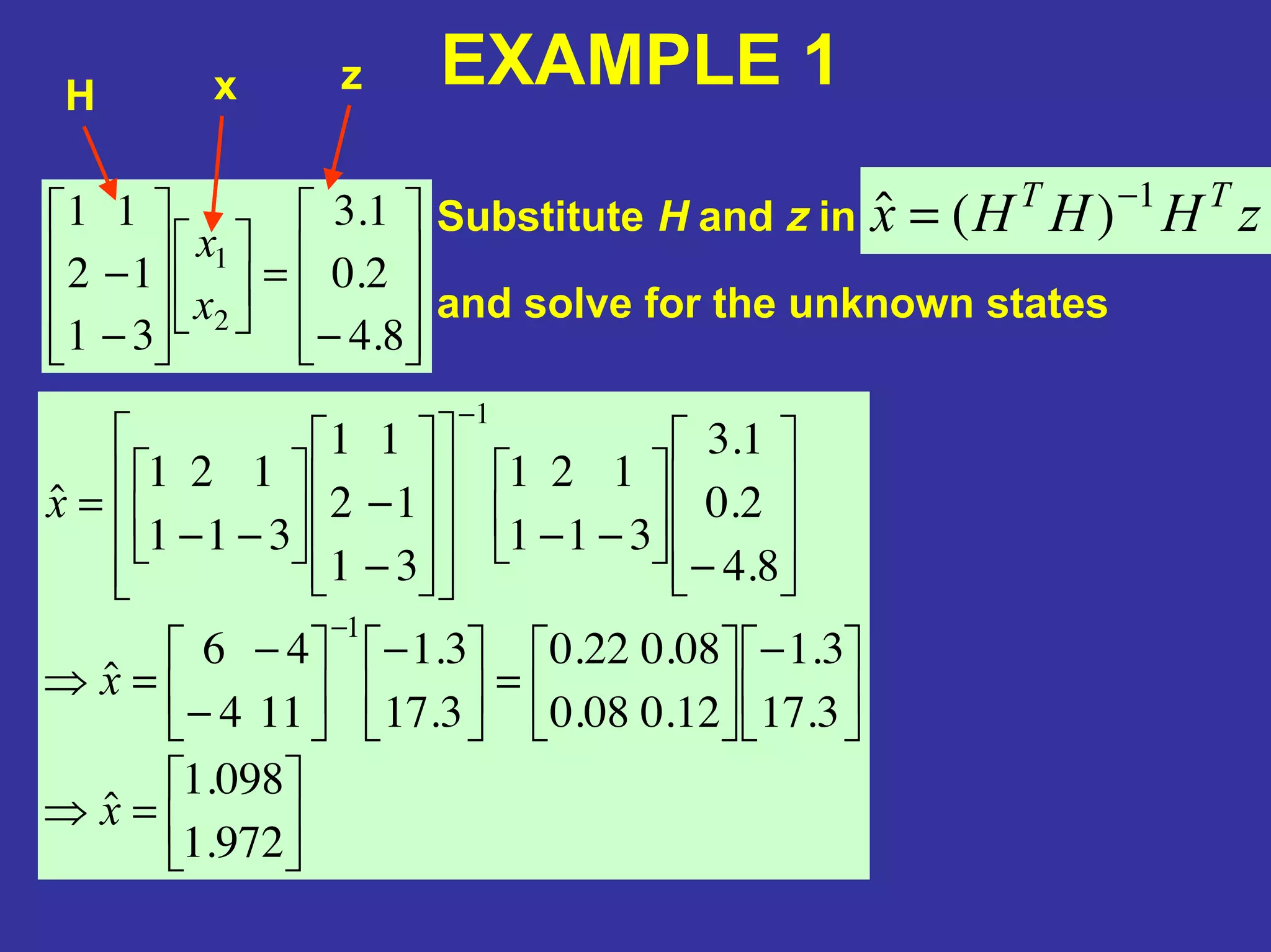
EXAMPLE 1H xz
zHHHx TT 1
)(ˆ −
=Substitute H and z in
and solve for the unknown states
=⇒
−
=
−
−
−
=⇒
−
−−
−
−
−−
=
−
−
972.1
098.1
ˆ
3.17
3.1
12.008.0
08.022.0
3.17
3.1
114
46
ˆ
8.4
2.0
1.3
311
121
31
12
11
311
121
ˆ
1
1
x
x
x
76.
EXAMPLE 1
To seehow much error we have in the estimated parameters,
we need to calculate the residual in a least squares sense
)ˆ()ˆ( xHzxHzrrJ TT
−−==
−
−
=
−
−
−
−=−=
018.0
224.0
03.0
8.4
2.0
1.3
972.1
098.1
31
12
11
ˆ zxHr
[ ] 0514.0
018.0
224.0
03.0
018.0224.003.0 =
−
−
−−=⇒ J
77.
WHY ARE ESTIMATORSNEEDED?
In power systems the state variables are
typically the voltage magnitudes and the relative
phase angles at the nodes of the system.
The available measurements may be voltage
magnitudes, current, real power, or reactive
power.
The estimator uses these noisy, imperfect
measurements to produce a best estimate for
the desired states.
78.
WHY ARE ESTIMATORSNEEDED?
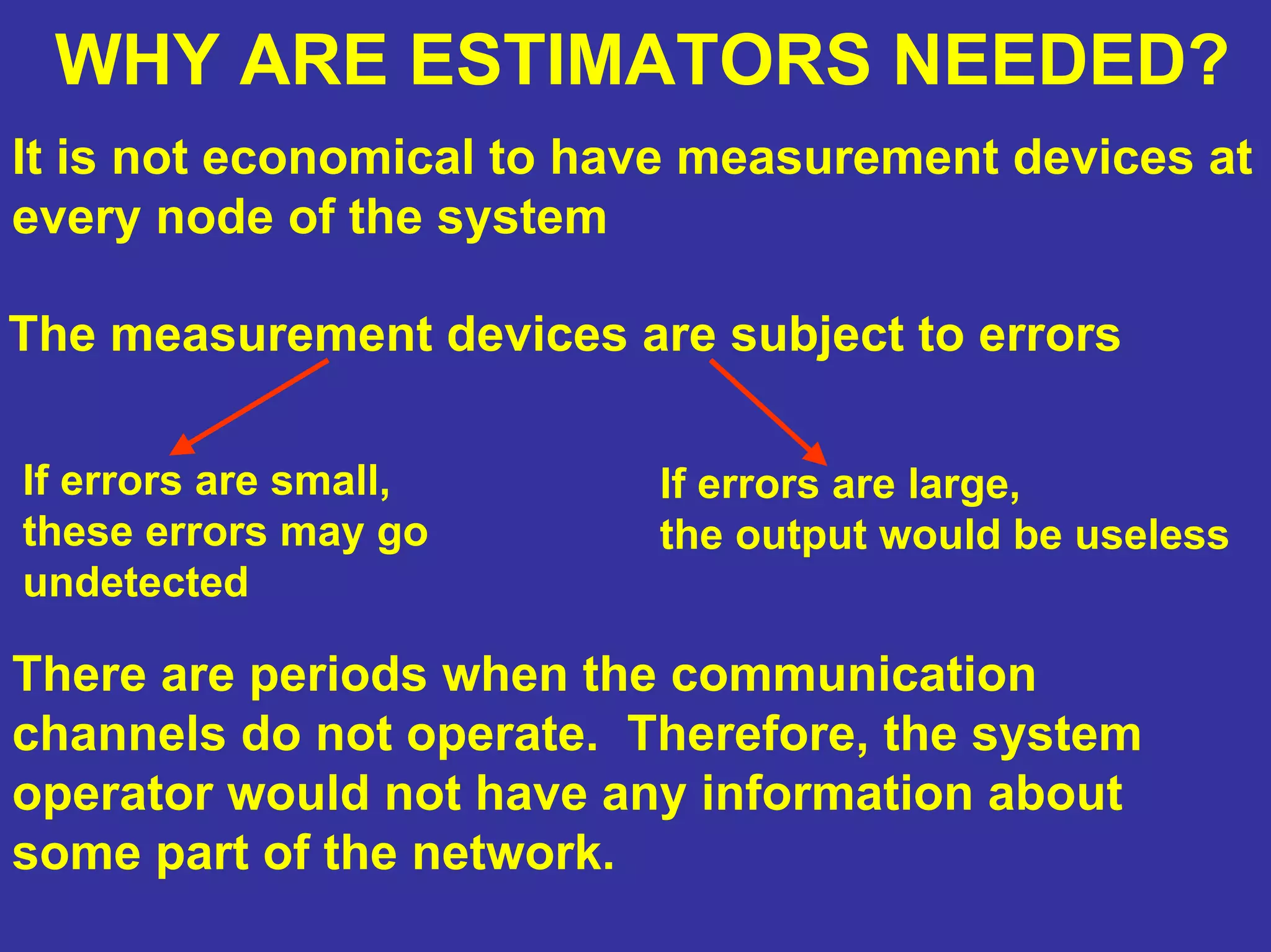
It is not economical to have measurement devices at
every node of the system
If errors are small,
these errors may go
undetected
The measurement devices are subject to errors
If errors are large,
the output would be useless
There are periods when the communication
channels do not operate. Therefore, the system
operator would not have any information about
some part of the network.
79.
HOW DOES THEESTIMATOR HELP?
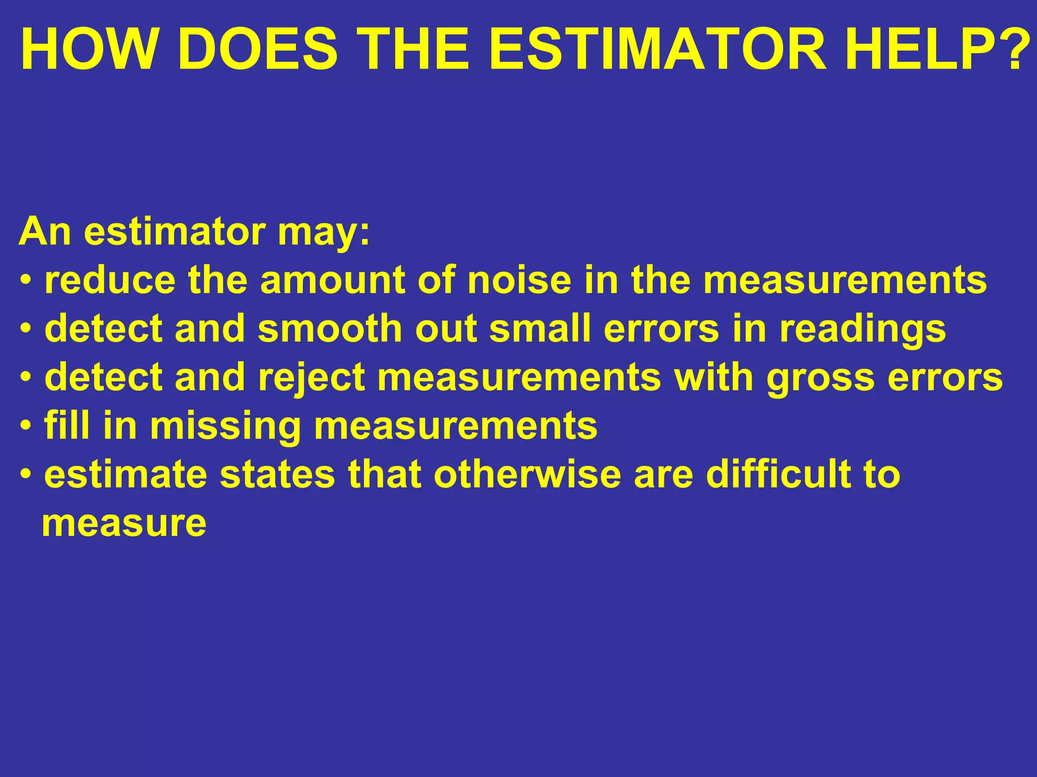
An estimator may:
• reduce the amount of noise in the measurements
• detect and smooth out small errors in readings
• detect and reject measurements with gross errors
• fill in missing measurements
• estimate states that otherwise are difficult to
measure
80.
EXAMPLE 2
R1
R2
R3
V1
V2 V3
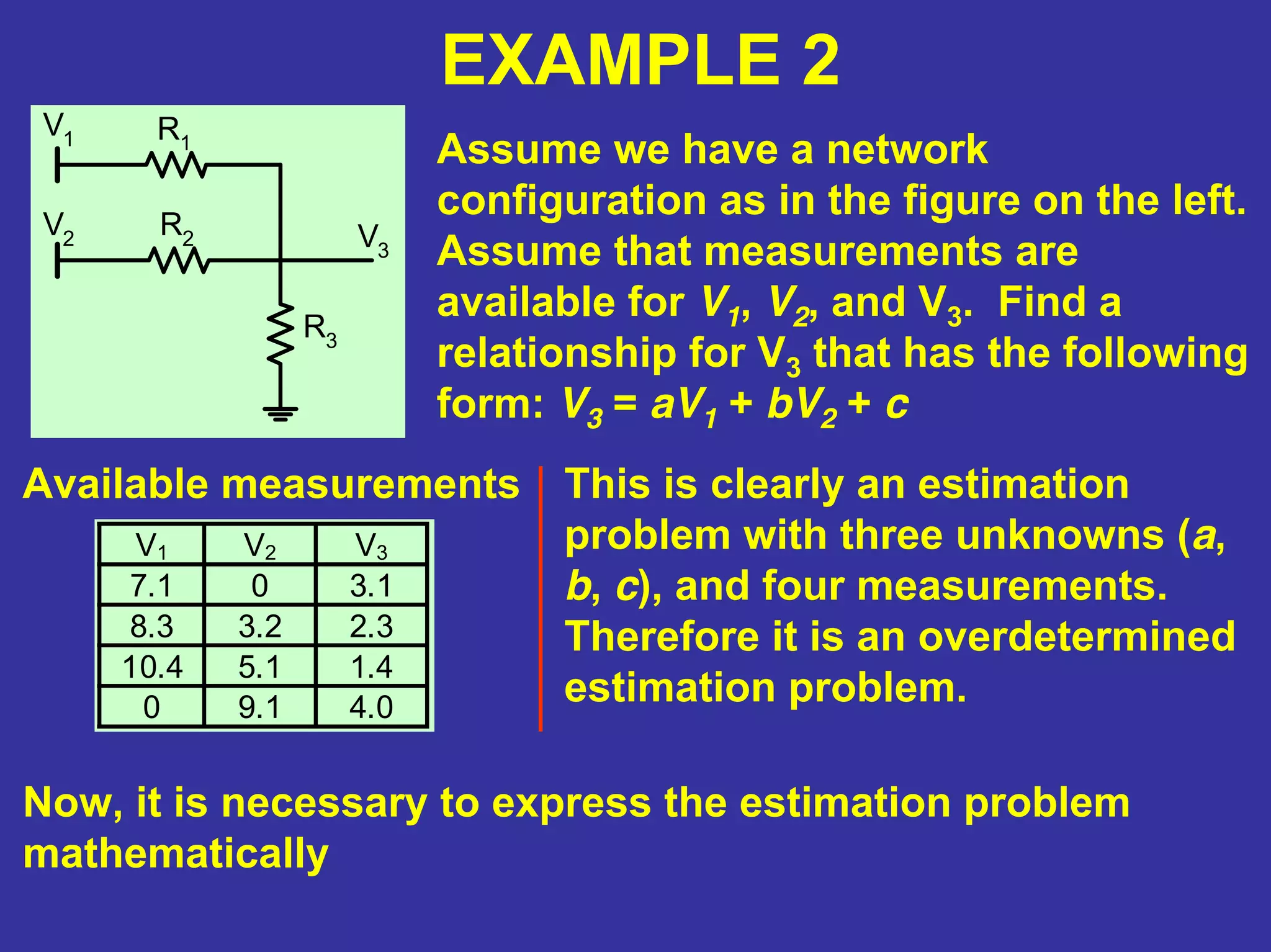
Assumewe have a network
configuration as in the figure on the left.
Assume that measurements are
available for V1, V2, and V3. Find a
relationship for V3 that has the following
form: V3 = aV1 + bV2 + c
Available measurements
V1 V2 V3
7.1 0 3.1
8.3 3.2 2.3
10.4 5.1 1.4
0 9.1 4.0
This is clearly an estimation
problem with three unknowns (a,
b, c), and four measurements.
Therefore it is an overdetermined
estimation problem.
Now, it is necessary to express the estimation problem
mathematically
81.
EXAMPLE 2
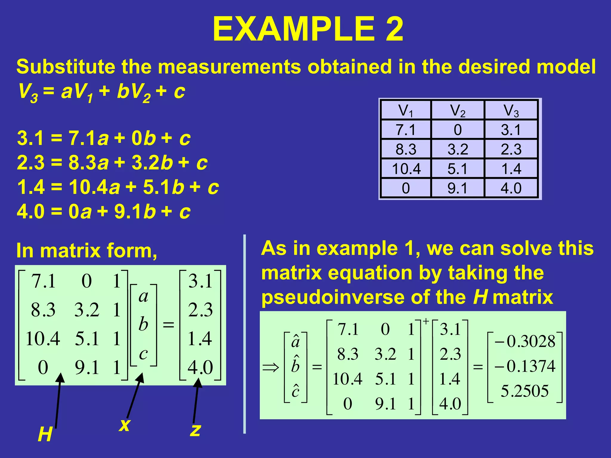
Substitute themeasurements obtained in the desired model
V3 = aV1 + bV2 + c
V1 V2 V3
7.1 0 3.1
8.3 3.2 2.3
10.4 5.1 1.4
0 9.1 4.0
3.1 = 7.1a + 0b + c
2.3 = 8.3a + 3.2b + c
1.4 = 10.4a + 5.1b + c
4.0 = 0a + 9.1b + c
In matrix form,
=
0.4
4.1
3.2
1.3
11.90
11.54.10
12.33.8
101.7
c
b
a
As in example 1, we can solve this
matrix equation by taking the
pseudoinverse of the H matrix
H
x z
−
−
==⇒
+
2505.5
1374.0
3028.0
0.4
4.1
3.2
1.3
11.90
11.54.10
12.33.8
101.7
ˆ
ˆ
ˆ
c
b
a
82.
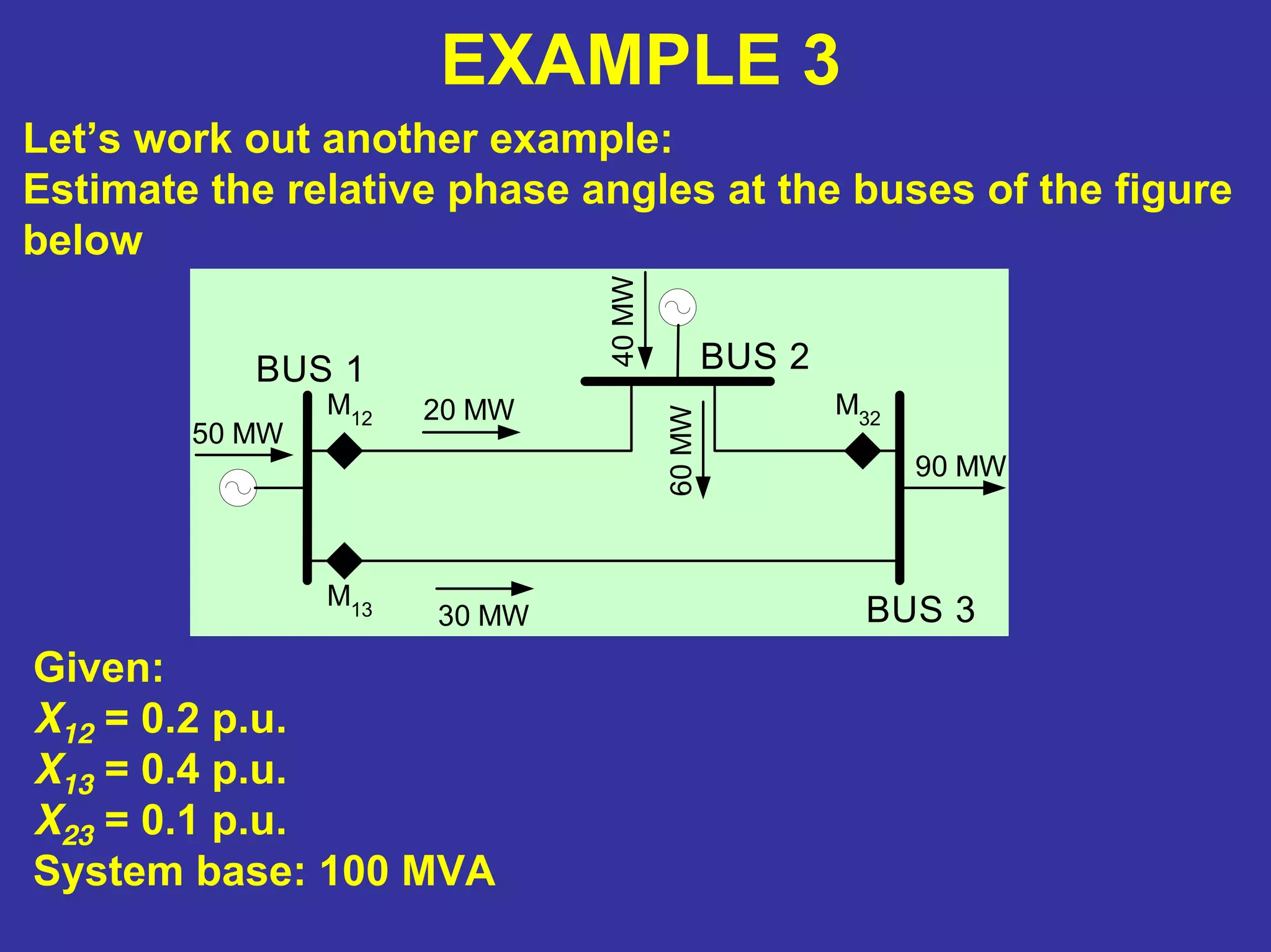
EXAMPLE 3
Let’s workout another example:
Estimate the relative phase angles at the buses of the figure
below
50 MW
M12
M13
M32
BUS 1 BUS 2
BUS 340MW
90 MW
20 MW
30 MW
60MWGiven:
X12 = 0.2 p.u.
X13 = 0.4 p.u.
X23 = 0.1 p.u.
System base: 100 MVA
83.
50 MW
M12
M13
M32
BUS 1BUS 2
BUS 3
40MW
90 MW
20 MW
30 MW 60MW
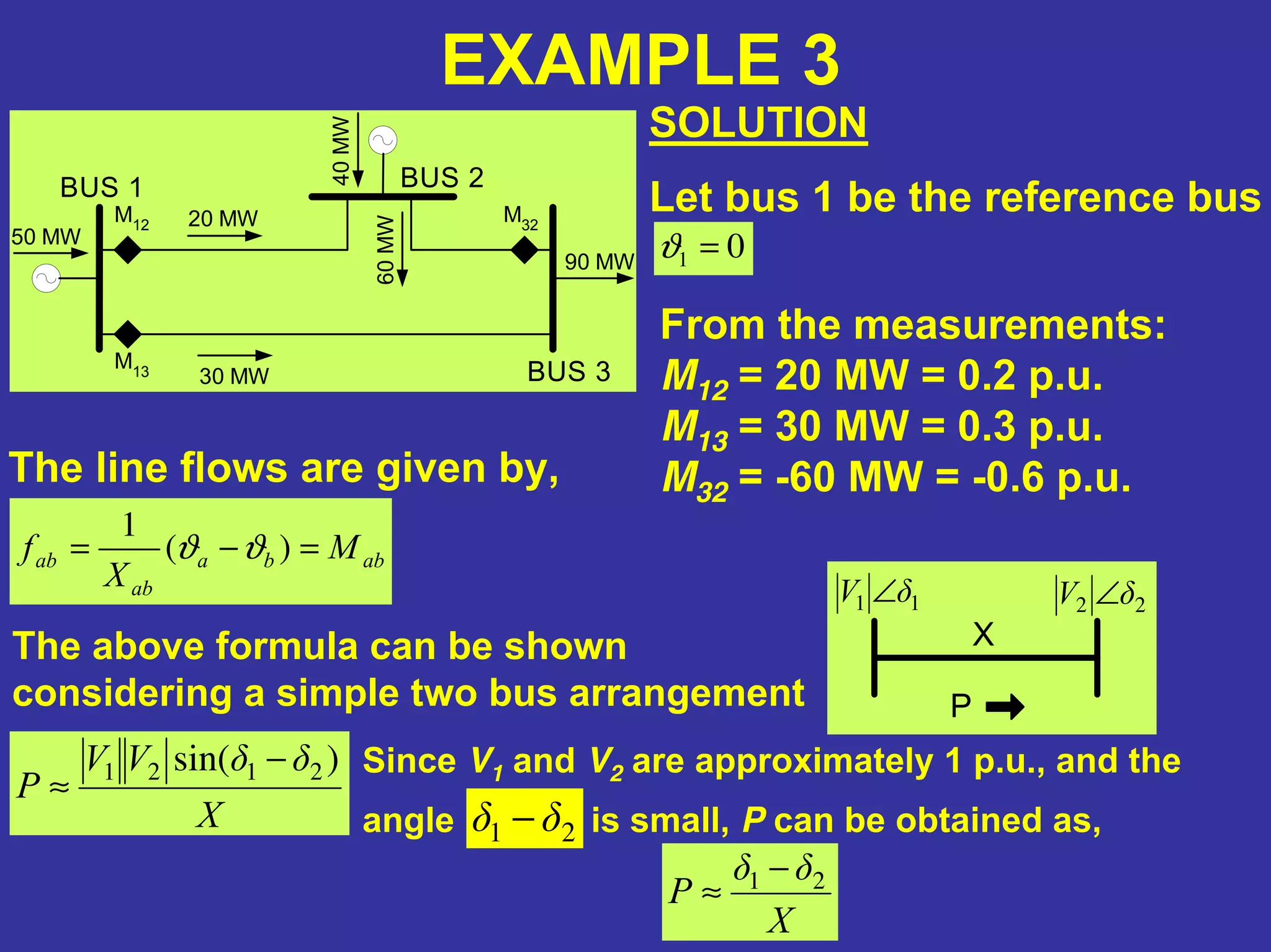
EXAMPLE 3
SOLUTION
Let bus 1 be the reference bus
01 =ϑ
From the measurements:
M12 = 20 MW = 0.2 p.u.
M13 = 30 MW = 0.3 p.u.
M32 = -60 MW = -0.6 p.u.The line flows are given by,
abba
ab
ab M
X
f =−= )(
1
ϑϑ
The above formula can be shown
considering a simple two bus arrangement
11 δV ∠ 22 δV ∠
X
P
X
δδVV
P
)sin( 2121 −
≈
Since V1 and V2 are approximately 1 p.u., and the
angle is small, P can be obtained as,21 δδ −
X
δδ
P 21 −
≈
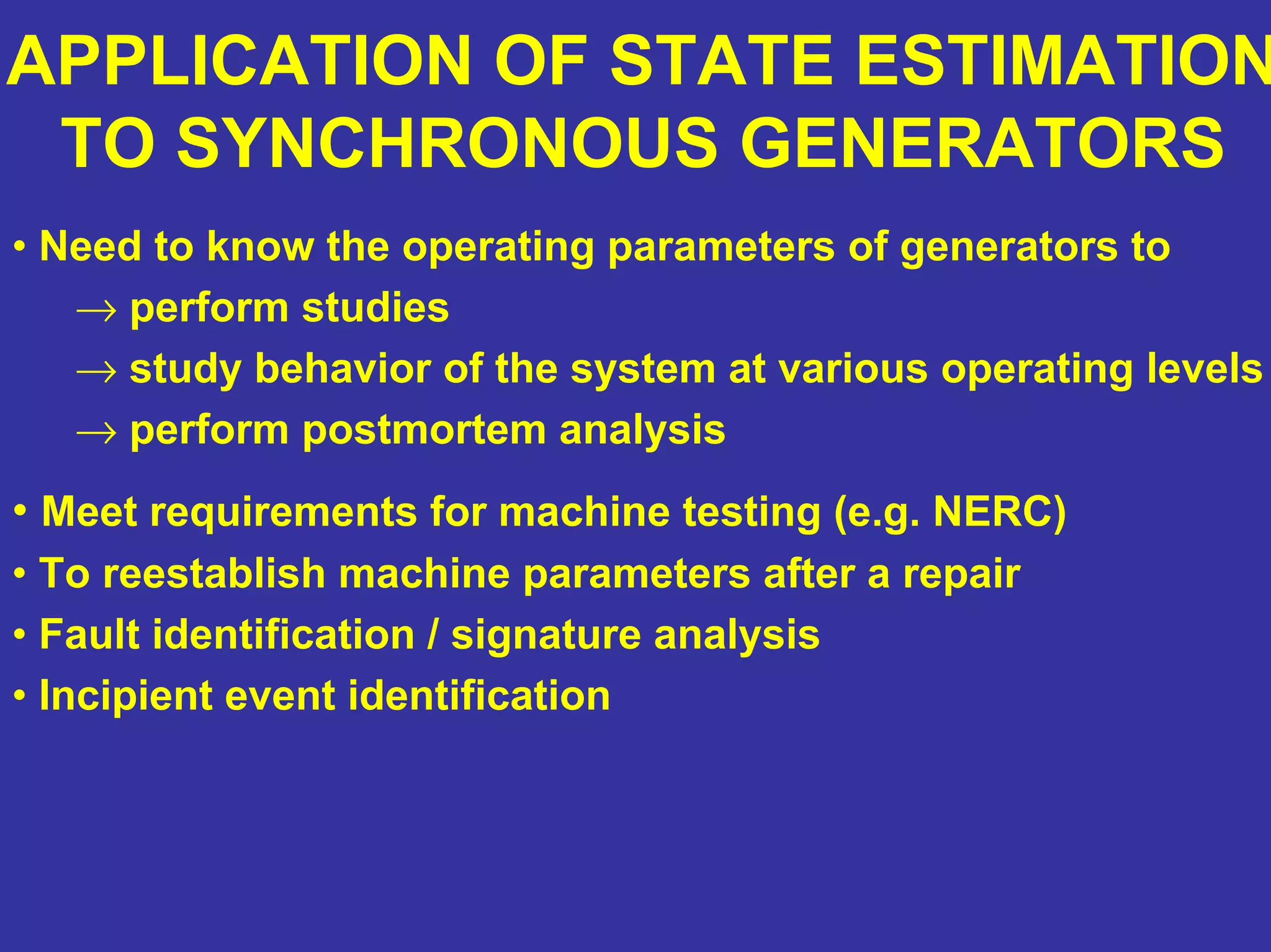
APPLICATION OF STATEESTIMATION
TO SYNCHRONOUS GENERATORS
• Need to know the operating parameters of generators to
→ perform studies
→ study behavior of the system at various operating levels
→ perform postmortem analysis
• Meet requirements for machine testing (e.g. NERC)
• To reestablish machine parameters after a repair
• Fault identification / signature analysis
• Incipient event identification
86.
APPLICATION OF STATEESTIMATION
TO SYNCHRONOUS GENERATORS
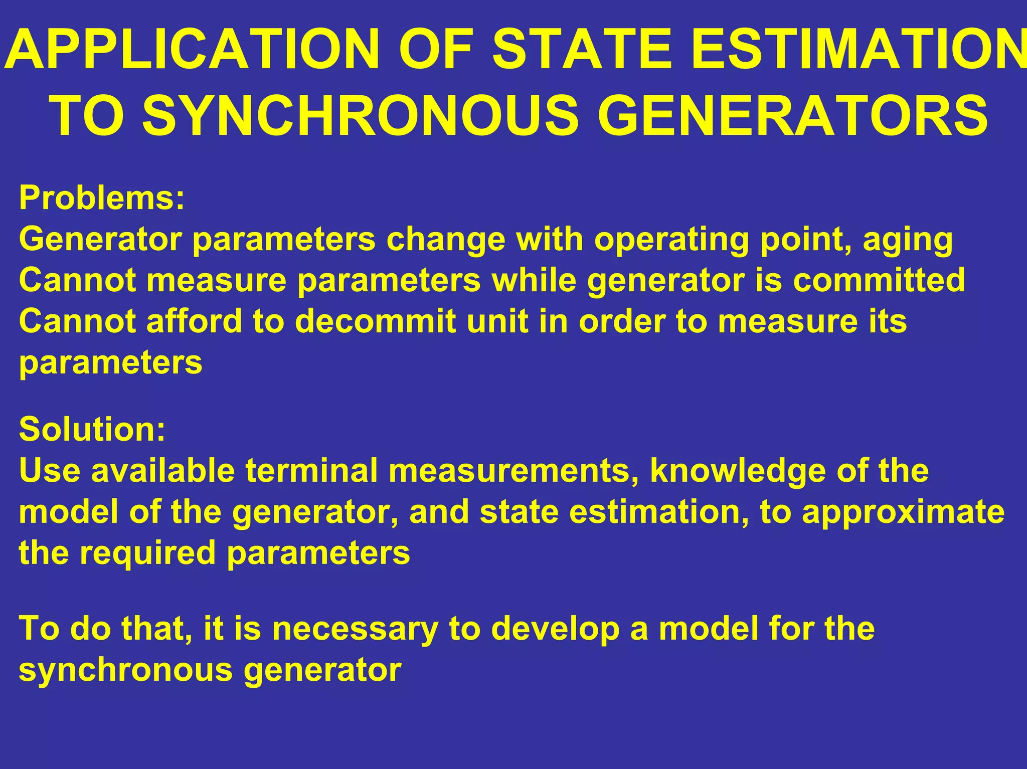
Problems:
Generator parameters change with operating point, aging
Cannot measure parameters while generator is committed
Cannot afford to decommit unit in order to measure its
parameters
Solution:
Use available terminal measurements, knowledge of the
model of the generator, and state estimation, to approximate
the required parameters
To do that, it is necessary to develop a model for the
synchronous generator
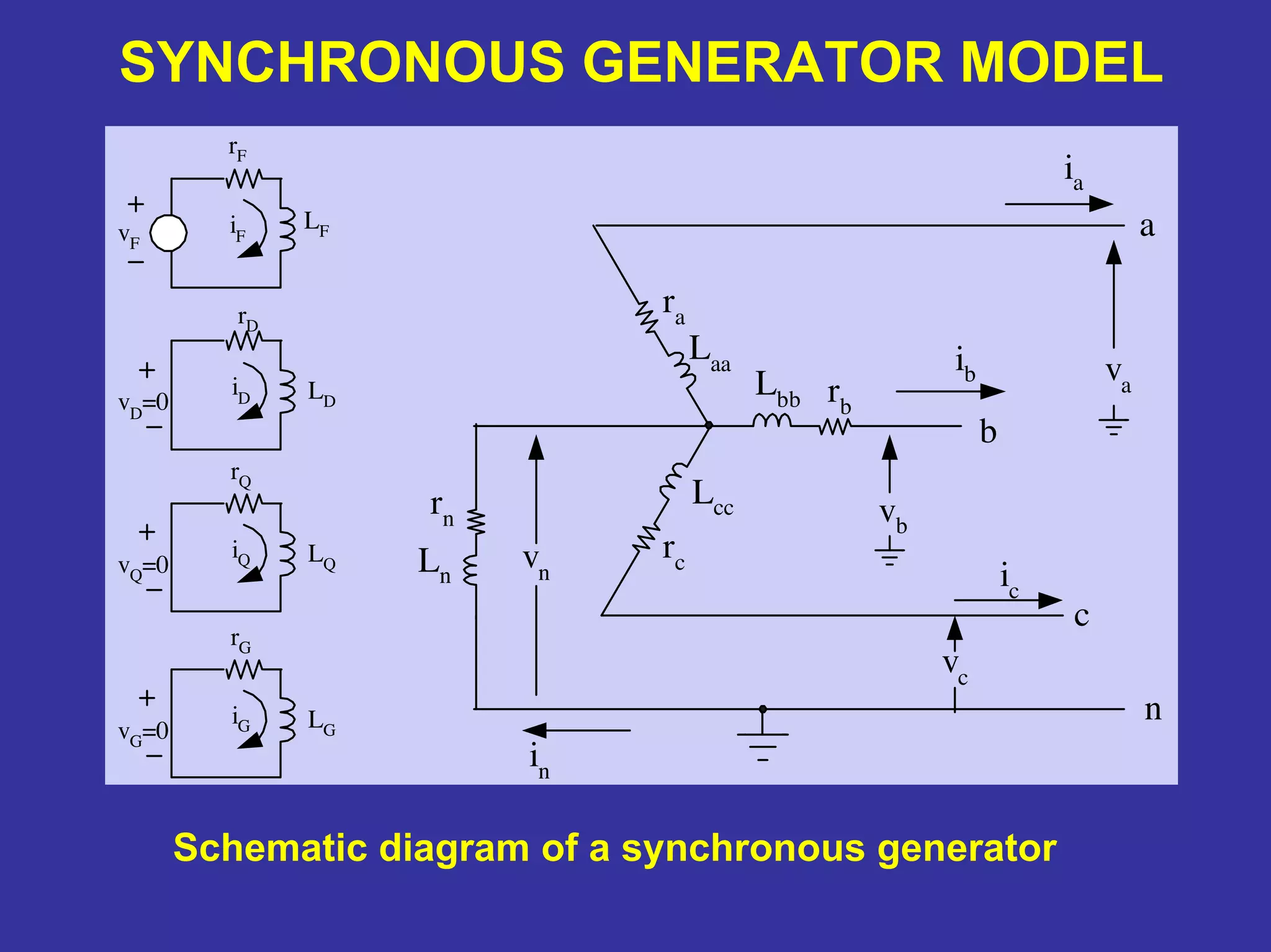
Schematic diagram ofa synchronous generator
SYNCHRONOUS GENERATOR MODEL
Lbb
rc
ra
rb
rn
Laa
Lcc
Ln
va
vb
vn ic
ib
ia
in
a
b
c
n
vc
rD
LDvD
=0
iD
rG
LGvG=0
iG
rF
LFiFvF
rQ
LQvQ=0
iQ
89.
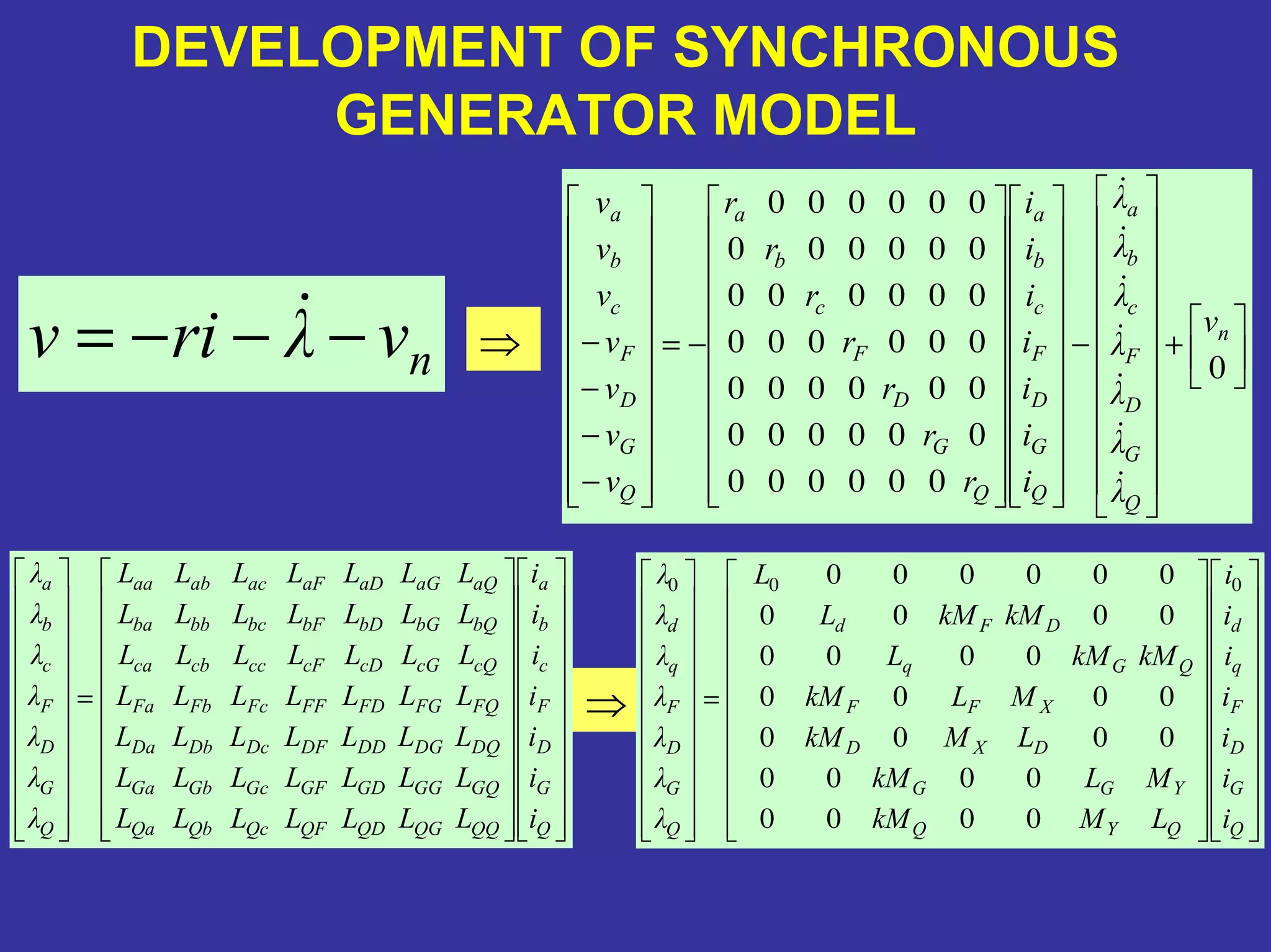
DEVELOPMENT OF SYNCHRONOUS
GENERATORMODEL
⇒
⇒nvλriv −−−= +−−=
−
−
−
−
0
000000
000000
000000
000000
000000
000000
000000
n
Q
G
D
F
c
b
a
Q
G
D
F
c
b
a
Q
G
D
F
c
b
a
Q
G
D
F
c
b
a
v
λ
λ
λ
λ
λ
λ
λ
i
i
i
i
i
i
i
r
r
r
r
r
r
r
v
v
v
v
v
v
v
=
Q
G
D
F
q
d
QYQ
YGG
DXD
XFF
QGq
DFd
Q
G
D
F
q
d
i
i
i
i
i
i
i
LMkM
MLkM
LMkM
MLkM
kMkML
kMkML
L
λ
λ
λ
λ
λ
λ
λ 000
0000
0000
0000
0000
0000
0000
000000
=
Q
G
D
F
c
b
a
QQQGQDQFQcQbQa
GQGGGDGFGcGbGa
DQDGDDDFDcDbDa
FQFGFDFFFcFbFa
cQcGcDcFcccbca
bQbGbDbFbcbbba
aQaGaDaFacabaa
Q
G
D
F
c
b
a
i
i
i
i
i
i
i
LLLLLLL
LLLLLLL
LLLLLLL
LLLLLLL
LLLLLLL
LLLLLLL
LLLLLLL
λ
λ
λ
λ
λ
λ
λ
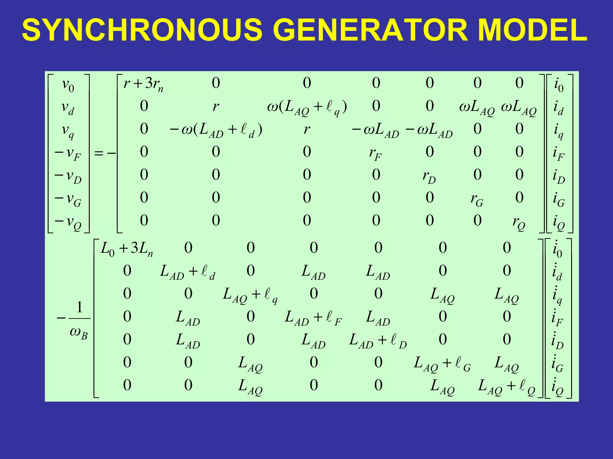
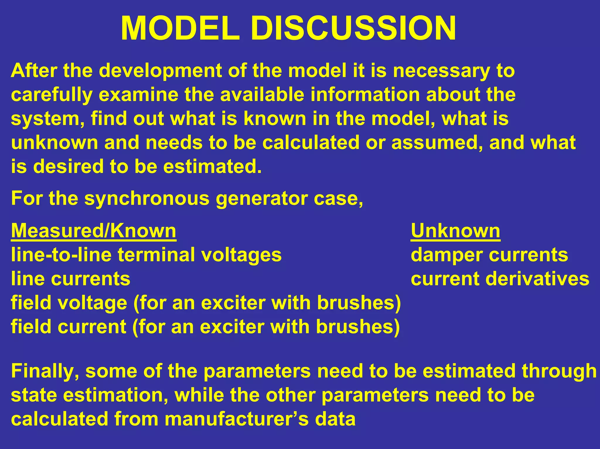
MODEL DISCUSSION
After thedevelopment of the model it is necessary to
carefully examine the available information about the
system, find out what is known in the model, what is
unknown and needs to be calculated or assumed, and what
is desired to be estimated.
For the synchronous generator case,
Measured/Known
line-to-line terminal voltages
line currents
field voltage (for an exciter with brushes)
field current (for an exciter with brushes)
Unknown
damper currents
current derivatives
Finally, some of the parameters need to be estimated through
state estimation, while the other parameters need to be
calculated from manufacturer’s data
93.
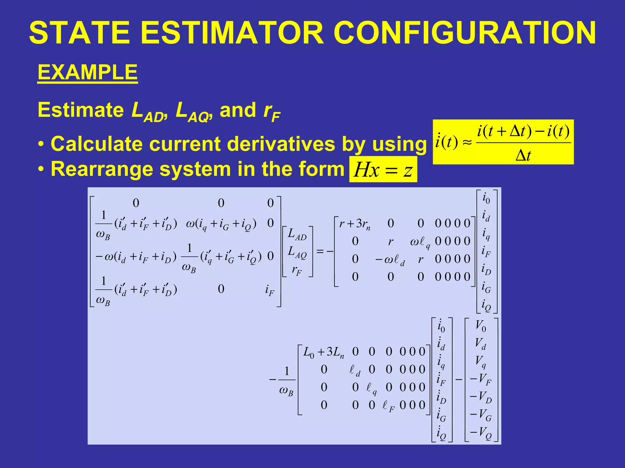
STATE ESTIMATOR CONFIGURATION
EXAMPLE
EstimateLAD, LAQ, and rF
t
titti
ti
∆
−∆+
≈
)()(
)(
−
−
−
−−
+
−
−
+
−=
′+′+′
′+′+′++−
++′+′+′
Q
G
D
F
q
d
Q
G
D
F
q
d
F
q
d
n
B
Q
G
D
F
q
d
d
q
n
F
AQ
AD
FDFd
B
QGq
B
DFd
QGqDFd
B
V
V
V
V
V
V
V
i
i
i
i
i
i
i
LL
ω
i
i
i
i
i
i
i
rω
ωr
rr
r
L
L
iiii
ω
iii
ω
iiiω
iiiωiii
ω
00
0
0
000000
000000
000000
0000003
1
0000000
00000
00000
0000003
0)(
1
0)(
1
)(
0)()(
1
000
• Calculate current derivatives by using
• Rearrange system in the form zHx =
94.
DEMONSTRATION OF PROTOTYPE
APPLICATIONFOR PARAMETER ESTIMATION
•Prototype application developed in Visual C++
•Portable, independent application
•Runs under Windows
•Purpose: Read measurements from DFR and use
manufacturer’s data to estimate generator
parameters
DIGITAL FAULT RECORDERS(DFRs)
A DFR is effectively a data acquisition system that is used to
monitor the performance of generation and transmission
equipment.
It is predominantly utilized to monitor system performance
during stressed conditions. For example, if a lightning
strikes a transmission line, the fault recognition by
protective relays and the fault clearance by circuit breakers
takes only about 50 to 83 ms.
This process is too fast for human intervention. Therefore,
the DFR saves a record of the desired signals (e.g. power
and current), and transmits this record to the central offices
over a modem, where a utility engineer can perform post-
event analysis to determine if the relays, circuit breakers and
other equipment functioned properly.
98.
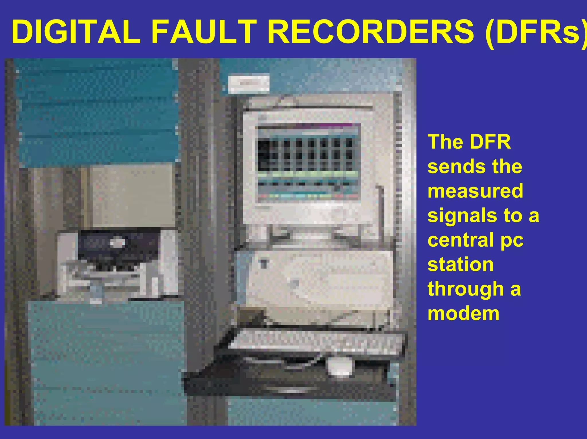
DIGITAL FAULT RECORDERS(DFRs)
The DFR
sends the
measured
signals to a
central pc
station
through a
modem
99.
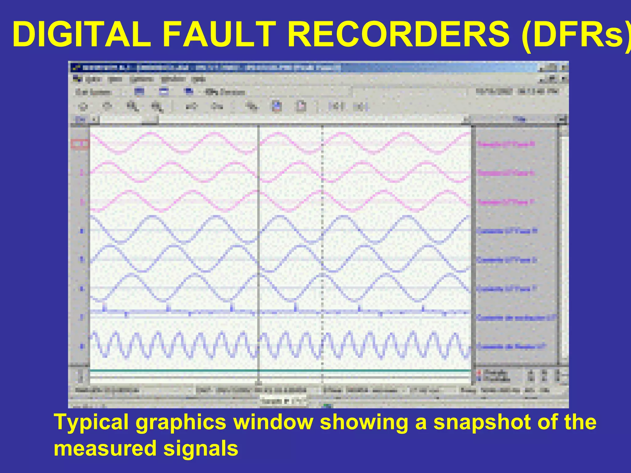
DIGITAL FAULT RECORDERS(DFRs)
Typical graphics window showing a snapshot of the
measured signals
100.
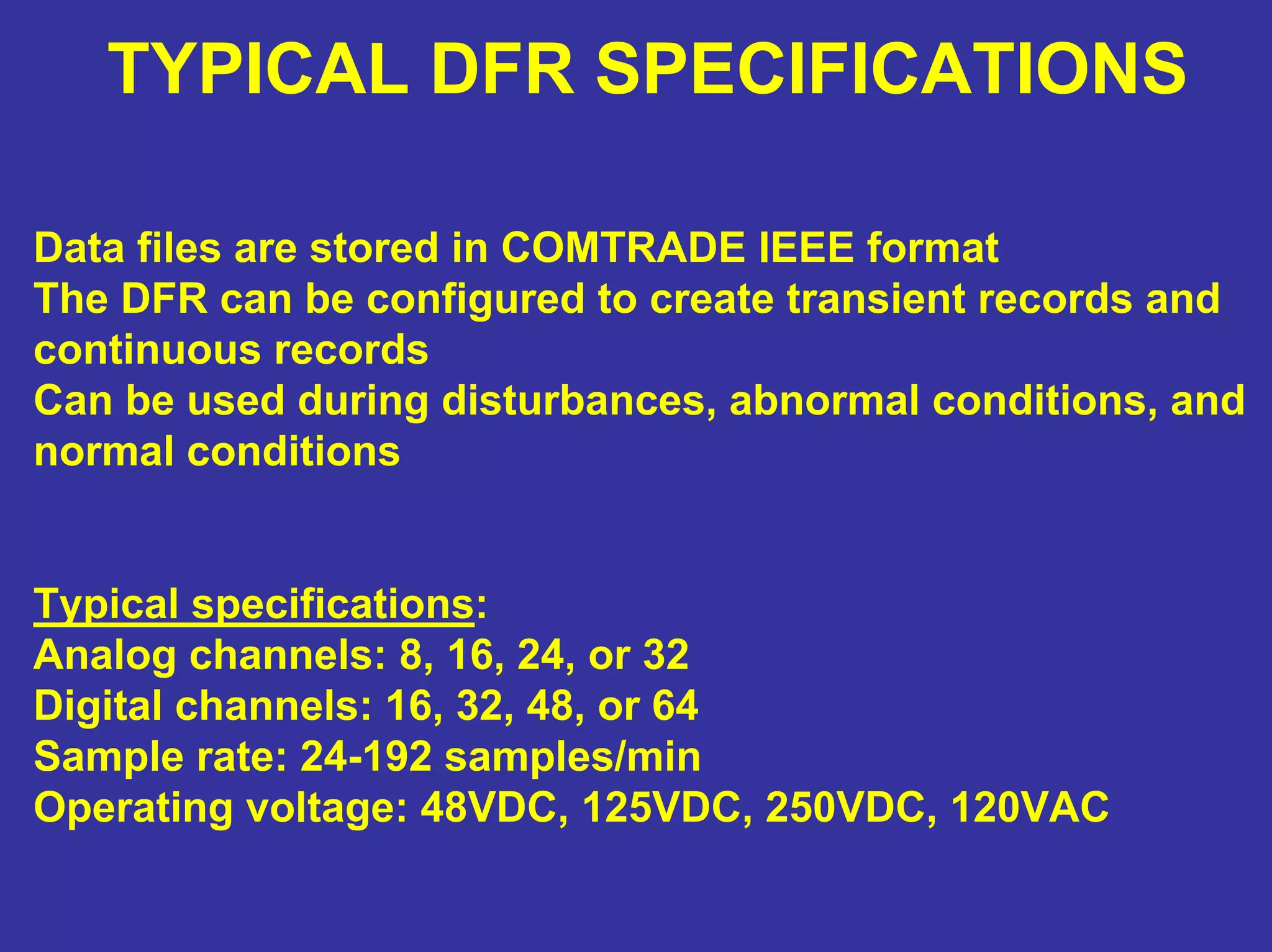
TYPICAL DFR SPECIFICATIONS
Datafiles are stored in COMTRADE IEEE format
The DFR can be configured to create transient records and
continuous records
Can be used during disturbances, abnormal conditions, and
normal conditions
Typical specifications:
Analog channels: 8, 16, 24, or 32
Digital channels: 16, 32, 48, or 64
Sample rate: 24-192 samples/min
Operating voltage: 48VDC, 125VDC, 250VDC, 120VAC
101.
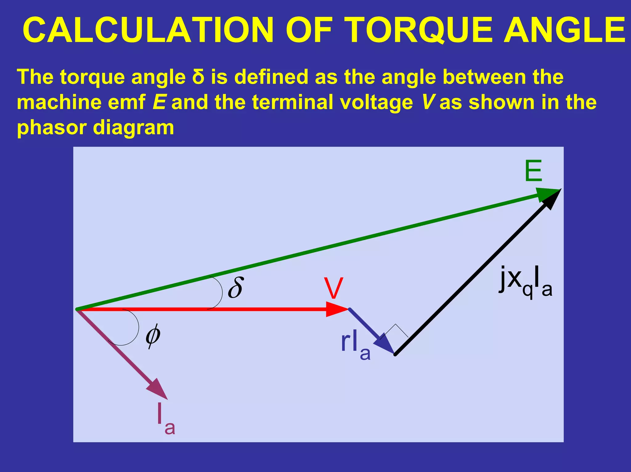
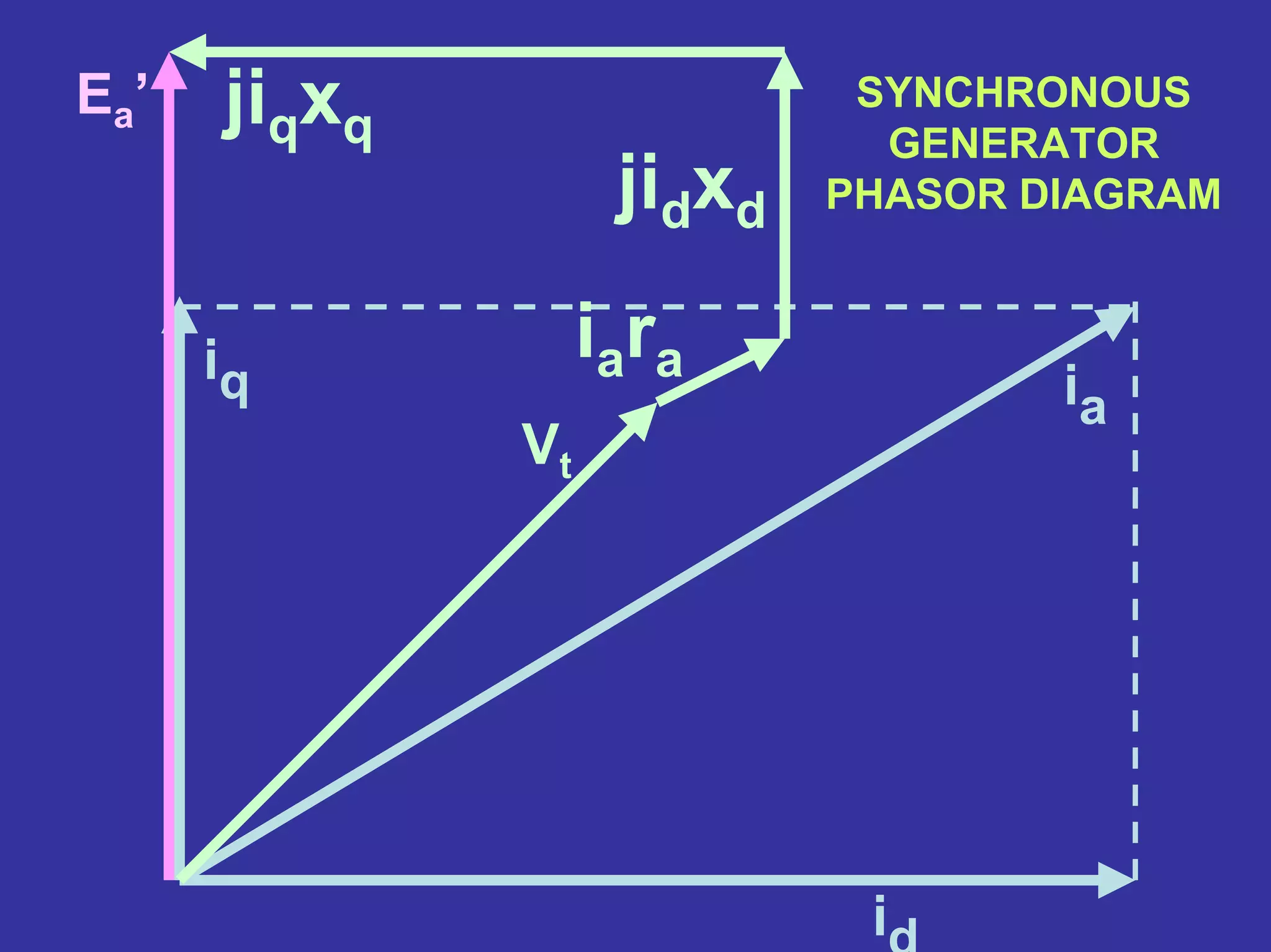
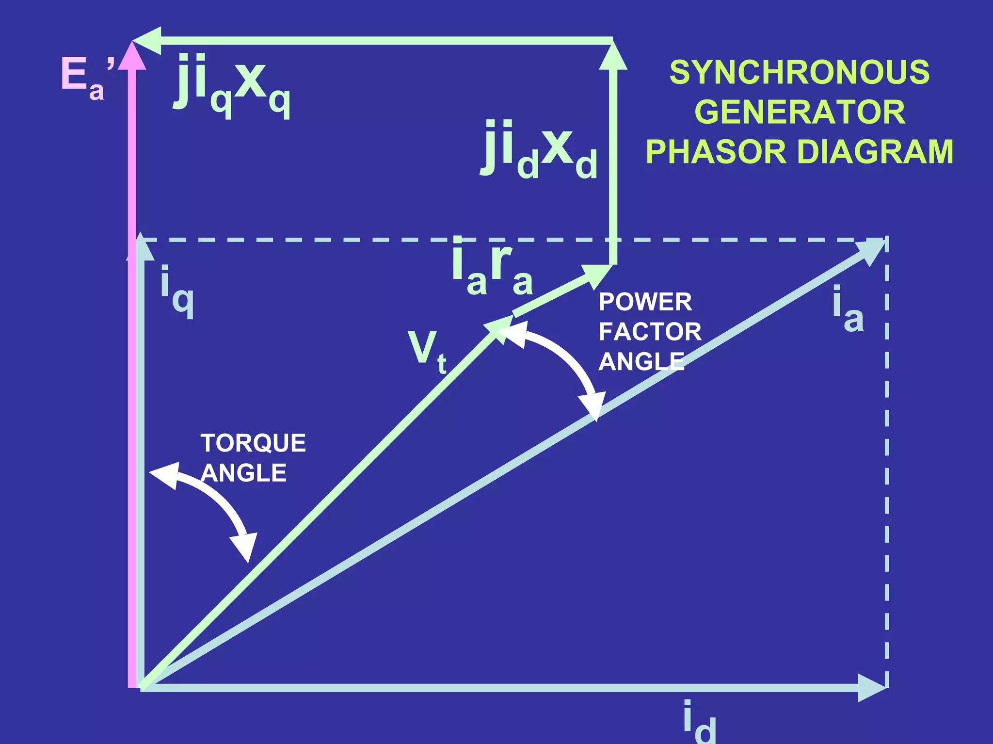
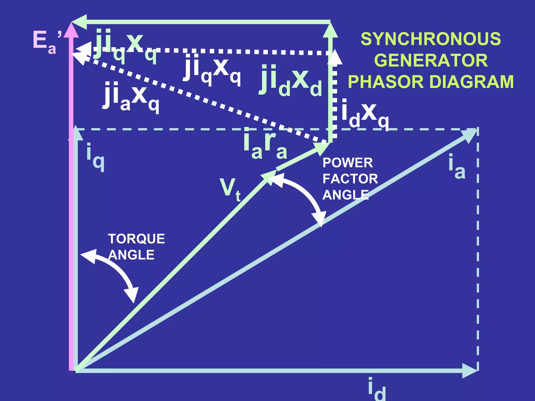
CALCULATION OF TORQUEANGLE
The torque angle δ is defined as the angle between the
machine emf E and the terminal voltage V as shown in the
phasor diagram
Ia
V
E
rIa
jxqIa
φ
δ
102.
CALCULATION OF TORQUEANGLE
The torque angle can be calculated in
different ways depending on what information
is available
Two ways to calculate the torque angle will be
shown:
1. Using line to line voltages and line currents
(stator frame of reference)
2. Using voltages and currents in the rotor frame of
reference (0dq quantities)
103.
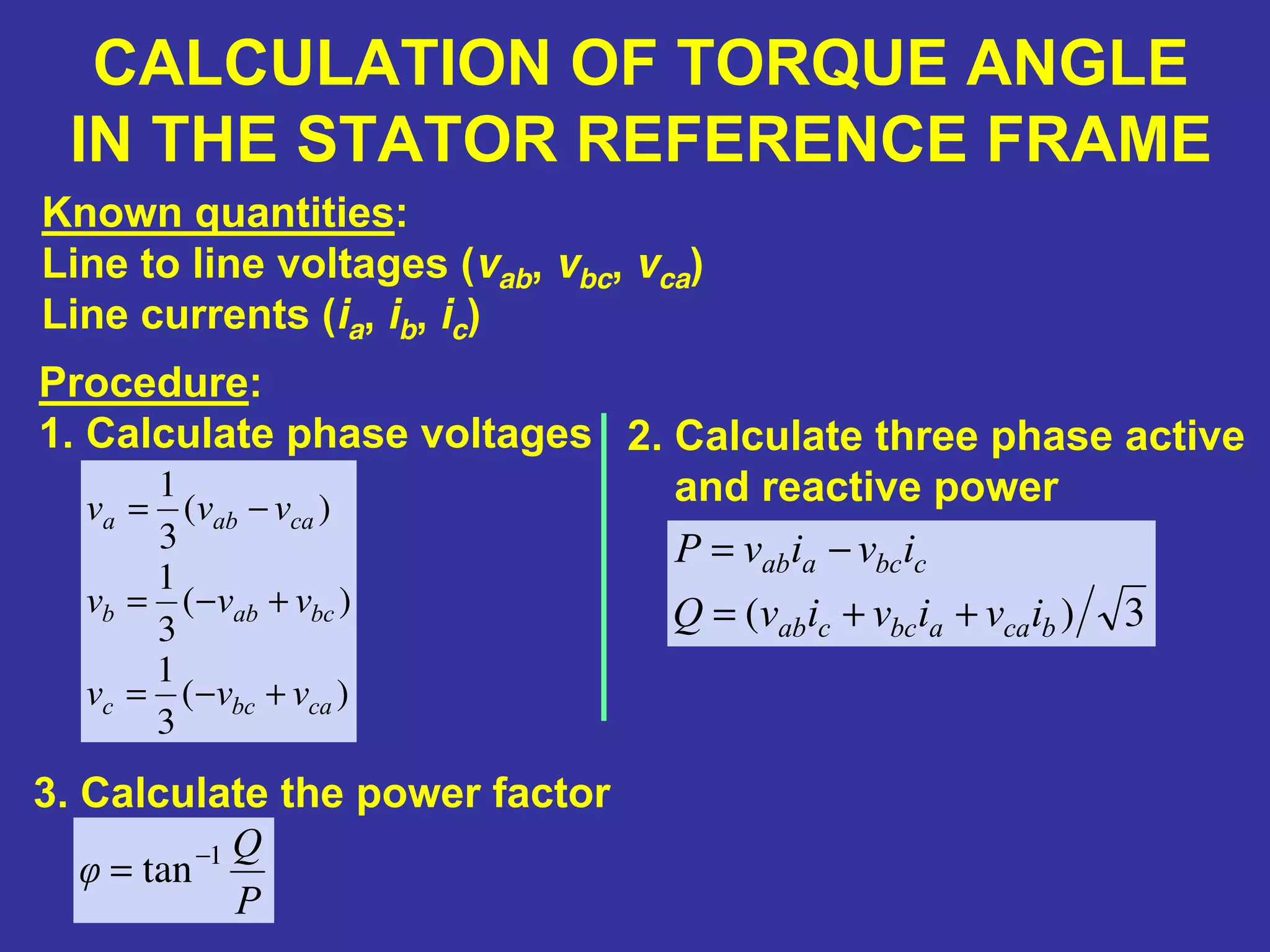
CALCULATION OF TORQUEANGLE
IN THE STATOR REFERENCE FRAME
Known quantities:
Line to line voltages (vab, vbc, vca)
Line currents (ia, ib, ic)
Procedure:
1. Calculate phase voltages
)(
3
1
)(
3
1
)(
3
1
cabcc
bcabb
caaba
vvv
vvv
vvv
+−=
+−=
−=
2. Calculate three phase active
and reactive power
3)( bcaabccab
cbcaab
ivivivQ
ivivP
++=
−=
3. Calculate the power factor
P
Q
φ 1
tan−
=
104.
CALCULATION OF TORQUEANGLE
IN THE STATOR REFERENCE FRAME
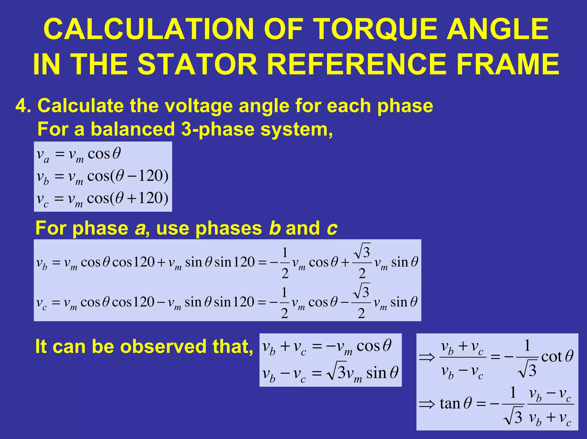
4. Calculate the voltage angle for each phase
For a balanced 3-phase system,
)120cos(
)120cos(
cos
+=
−=
=
θvv
θvv
θvv
mc
mb
ma
For phase a, use phases b and c
θvθvθvθvv
θvθvθvθvv
mmmmc
mmmmb
sin
2
3
cos
2
1
120sinsin120coscos
sin
2
3
cos
2
1
120sinsin120coscos
−−=−=
+−=+=
It can be observed that,
θvvv
θvvv
mcb
mcb
sin3
cos
=−
−=+
cb
cb
cb
cb
vv
vv
θ
θ
vv
vv
+
−
−=⇒
−=
−
+
⇒
3
1
tan
cot
3
1
105.
CALCULATION OF TORQUEANGLE
IN THE STATOR REFERENCE FRAME
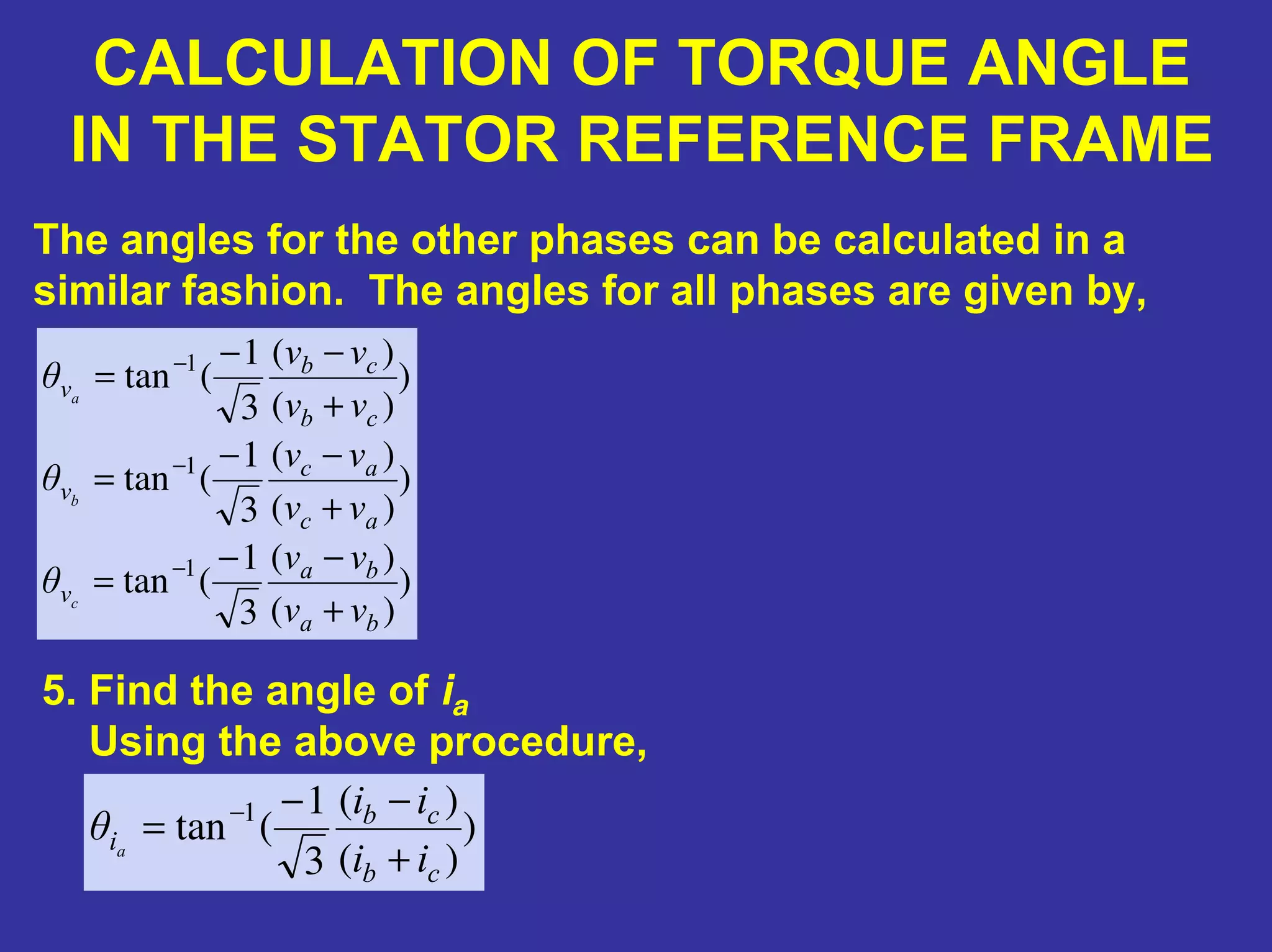
5. Find the angle of ia
Using the above procedure,
The angles for the other phases can be calculated in a
similar fashion. The angles for all phases are given by,
)
)(
)(
3
1
(tan
)
)(
)(
3
1
(tan
)
)(
)(
3
1
(tan
1
1
1
ba
ba
v
ac
ac
v
cb
cb
v
vv
vv
θ
vv
vv
θ
vv
vv
θ
c
b
a
+
−−
=
+
−−
=
+
−−
=
−
−
−
)
)(
)(
3
1
(tan 1
cb
cb
i
ii
ii
θ a
+
−−
= −
106.
CALCULATION OF TORQUEANGLE
IN THE STATOR REFERENCE FRAME
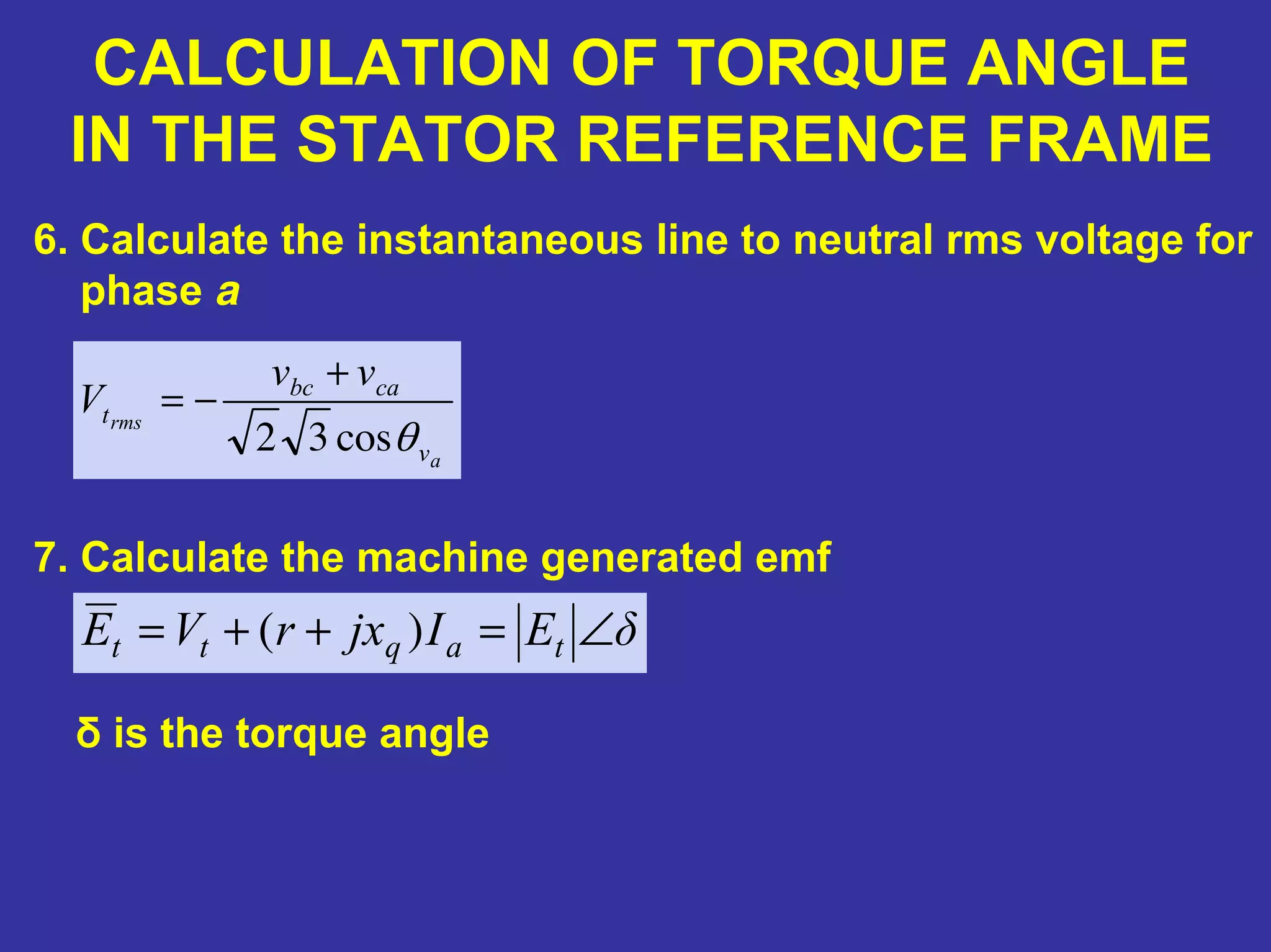
6. Calculate the instantaneous line to neutral rms voltage for
phase a
7. Calculate the machine generated emf
a
rms
v
cabc
t
vv
V
θcos32
+
−=
δEIjxrVE taqtt ∠=++= )(
δ is the torque angle
107.
CALCULATION OF TORQUEANGLE
IN THE ROTOR REFERENCE FRAME
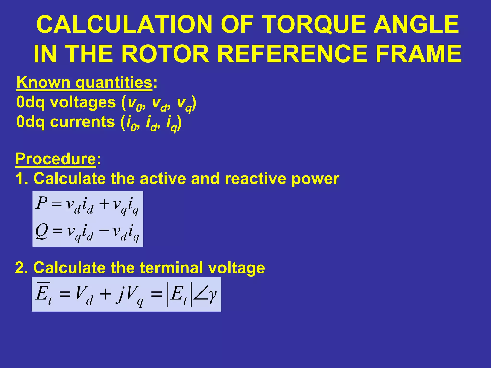
Known quantities:
0dq voltages (v0, vd, vq)
0dq currents (i0, id, iq)
Procedure:
1. Calculate the active and reactive power
qddq
qqdd
ivivQ
ivivP
−=
+=
2. Calculate the terminal voltage
γEjVVE tqdt ∠=+=
108.
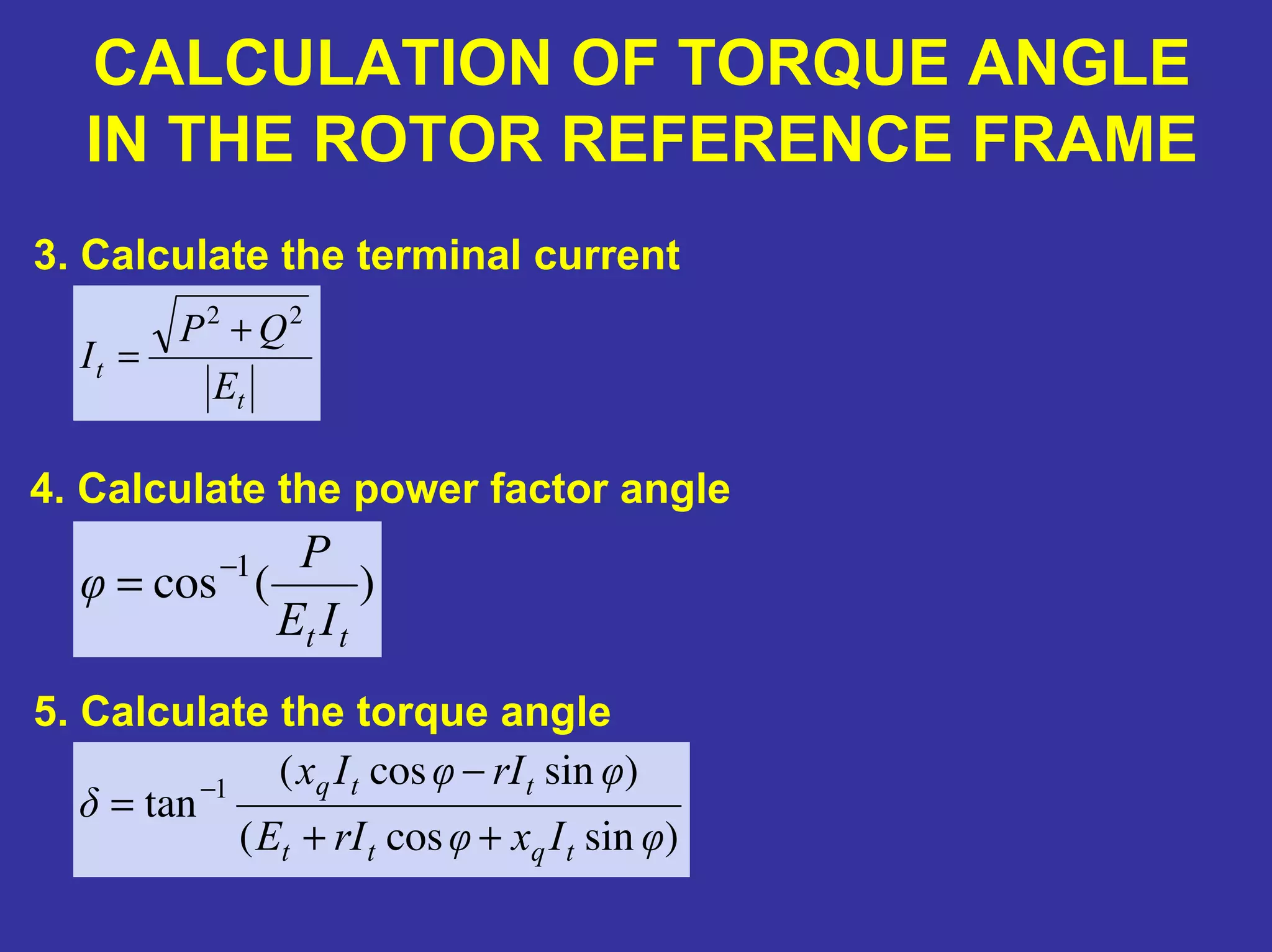
CALCULATION OF TORQUEANGLE
IN THE ROTOR REFERENCE FRAME
3. Calculate the terminal current
t
t
E
QP
I
22
+
=
4. Calculate the power factor angle
5. Calculate the torque angle
)(cos 1
tt IE
P
φ −
=
)sincos(
)sincos(
tan 1
φIxφrIE
φrIφIx
δ
tqtt
ttq
++
−
= −
![Synchronous Machines
Active power will flow when there is a phase
difference between Vsend and Vreceive.
This is because when there is a phase
difference, there will be a voltage difference
across the reactance jx, and therefore there
will be a current flowing in jx. After some
arithmetic
Psent = [|Vsend|] [|Vreceive|] sin(torque angle) / x](https://image.slidesharecdn.com/synchronousmachinespresentation-160401012745/75/Synchronous-machines-14-2048.jpg)
![EXAMPLE 1
To see how much error we have in the estimated parameters,
we need to calculate the residual in a least squares sense
)ˆ()ˆ( xHzxHzrrJ TT
−−==
−
−
=
−
−
−
−=−=
018.0
224.0
03.0
8.4
2.0
1.3
972.1
098.1
31
12
11
ˆ zxHr
[ ] 0514.0
018.0
224.0
03.0
018.0224.003.0 =
−
−
−−=⇒ J](https://image.slidesharecdn.com/synchronousmachinespresentation-160401012745/75/Synchronous-machines-76-2048.jpg)
![+−
+−=
)
3
2sin()
3
2sin(sin
)
3
2cos()
3
2cos(cos
2
1
2
1
2
1
3
2
πϑπϑϑ
πϑπϑϑP
abcdq Pii =0 abcdq Pvv =0abcdq λPλ =0
DEVELOPMENT OF SYNCHRONOUS
GENERATOR MODEL
[ ] [ ]−−=
14
130
77
14
130
77
14
130
xFDGQ
xdq
x
xFDGQ
xdq
x
xFDGQ
xdq
i
i
L
i
i
R
v
v
Resulting model:](https://image.slidesharecdn.com/synchronousmachinespresentation-160401012745/75/Synchronous-machines-90-2048.jpg)