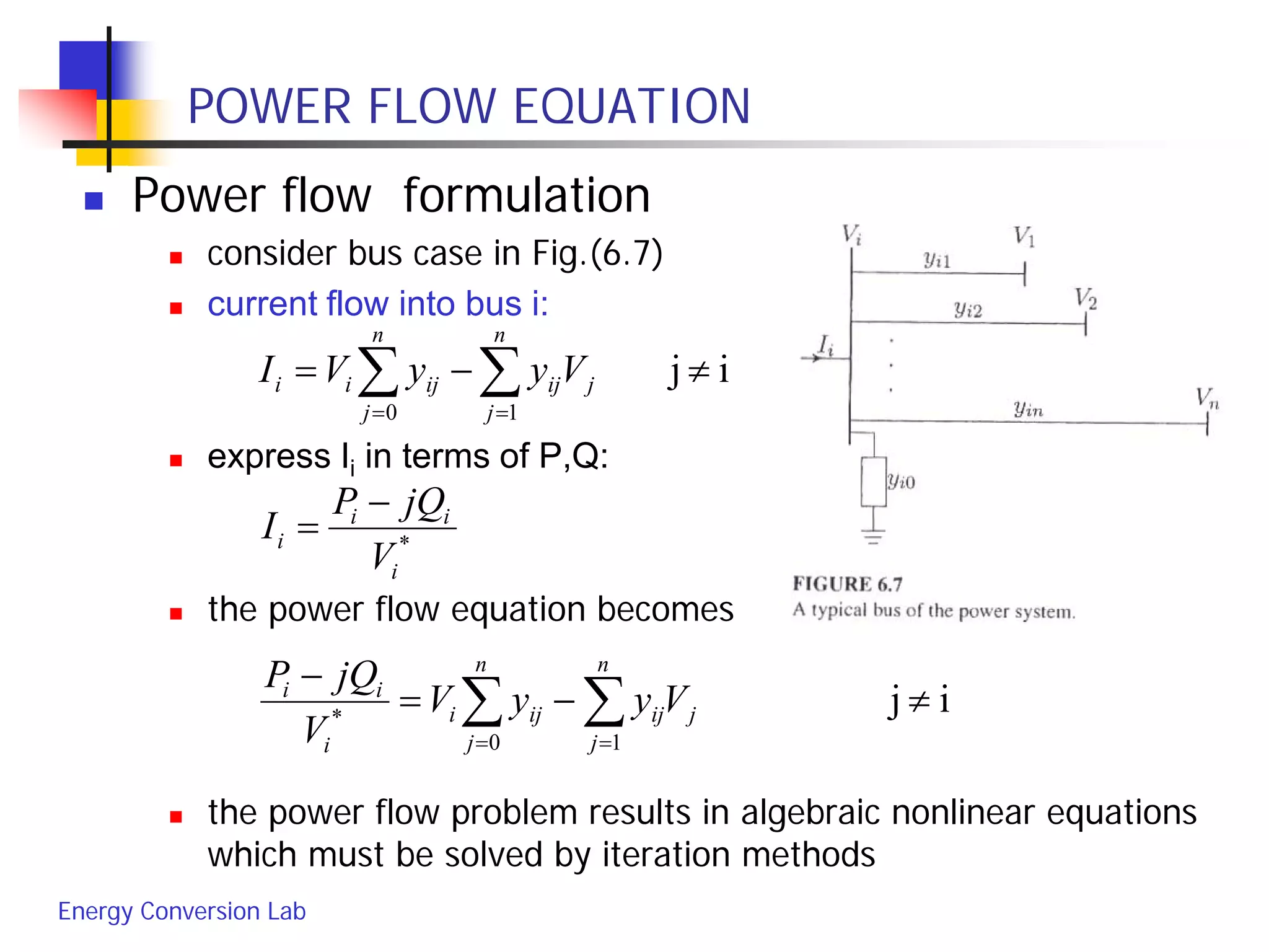
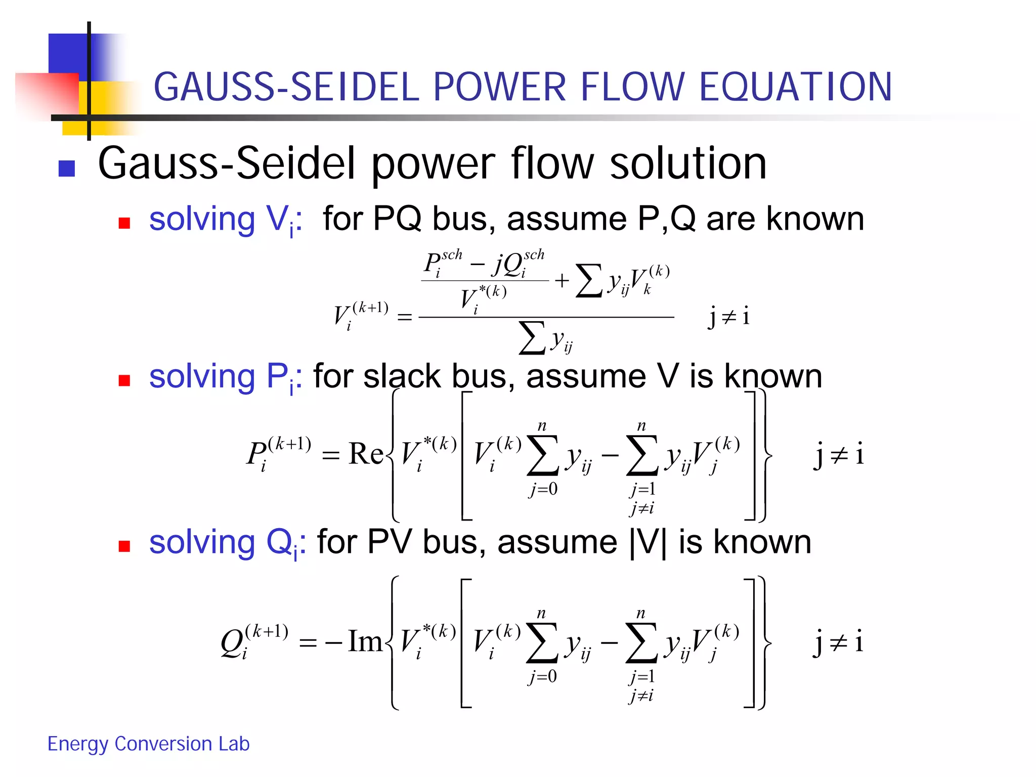
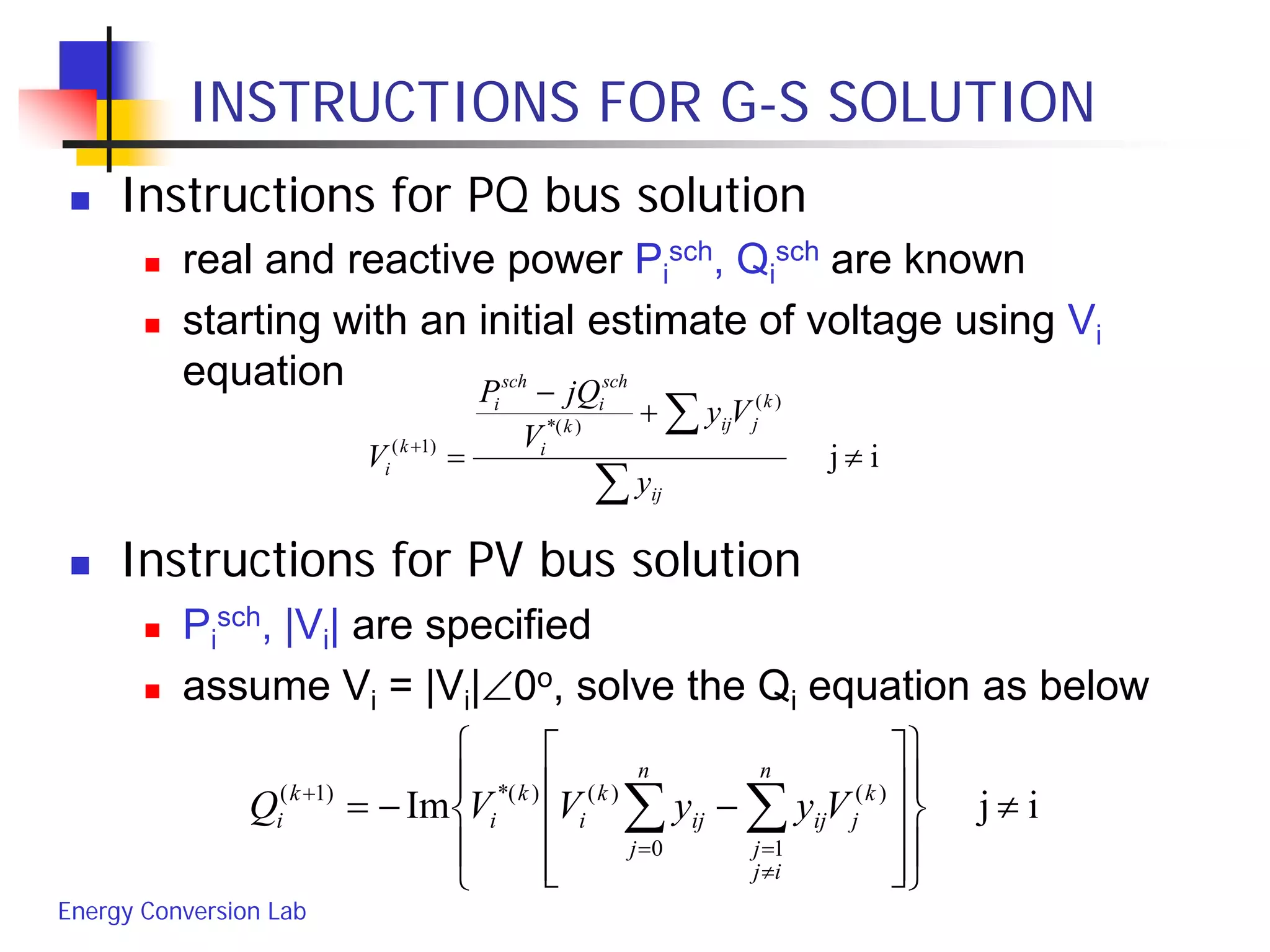
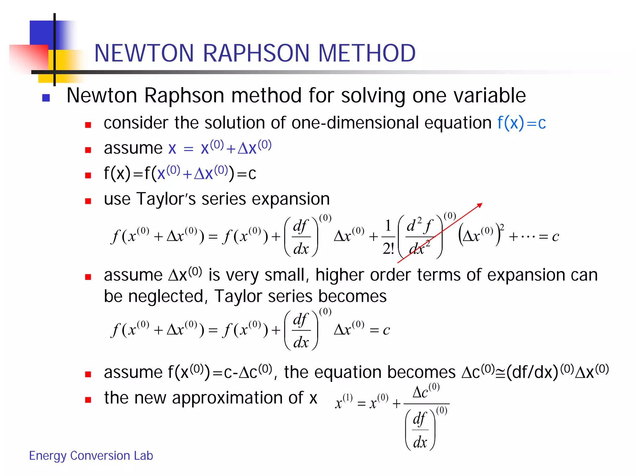
The document discusses power flow analysis and solutions using the Gauss-Seidel method. It describes setting up the bus admittance matrix and node-voltage equations based on impedance values between nodes. The Gauss-Seidel method is then used to iteratively solve the nonlinear power flow equations to determine bus voltages and power flows by updating the solution for one variable at a time. Instructions are provided on applying the method to different bus types including slack, PQ and PV buses.
![Energy Conversion Lab
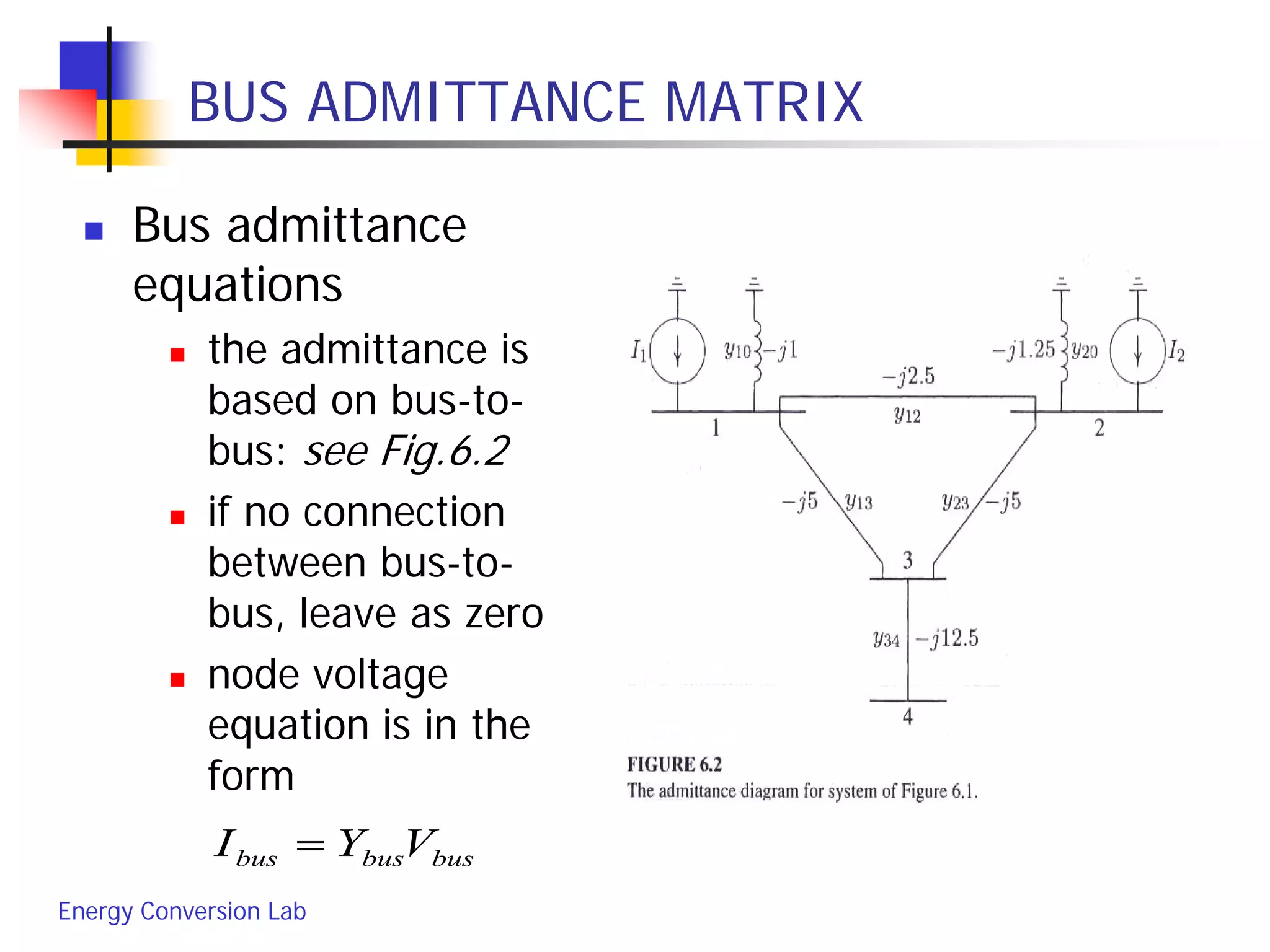
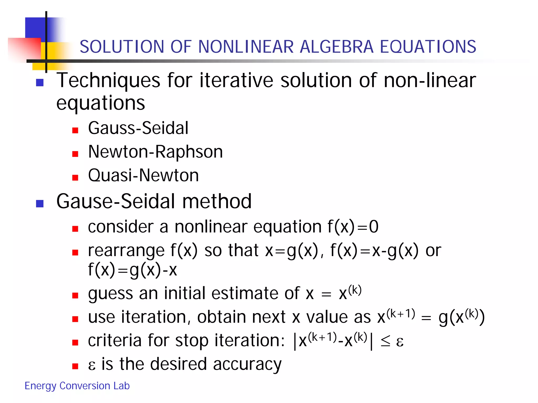
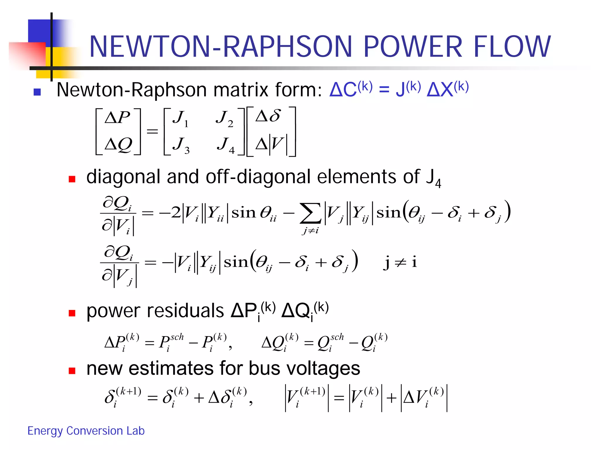
GAUSE-SEIDAL METHOD
Nature of Gause-Seidal method
solution: if initial estimate x is within convergent
region, solution will converge in zigzag fashion to one
of the roots
no solution: if initial estimate x is outside convergent
region, process will diverge, no solution found
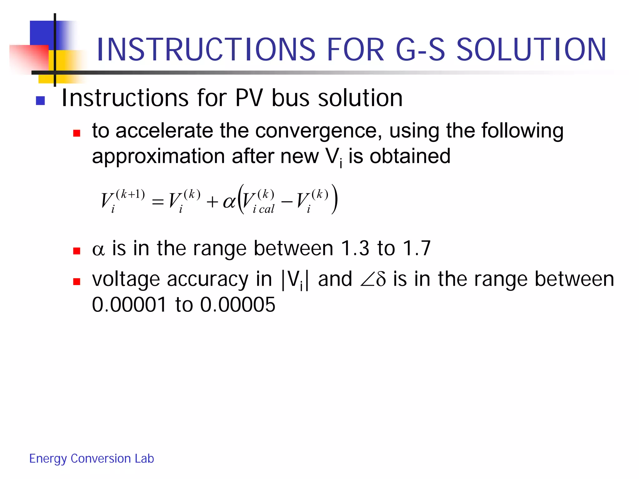
in some case, an acceleration factor α is added to
improve the rate of convergence:
x(k+1) = x(k) +α[g(x(k))-x(k)], where α>1
acceleration factor should not too large to produce
overshoot
see Ex.(6.3) for the acceleration factor used](https://image.slidesharecdn.com/apschap9powerflow-150705002455-lva1-app6891/75/APSA-LEC-9-9-2048.jpg)
![Energy Conversion Lab
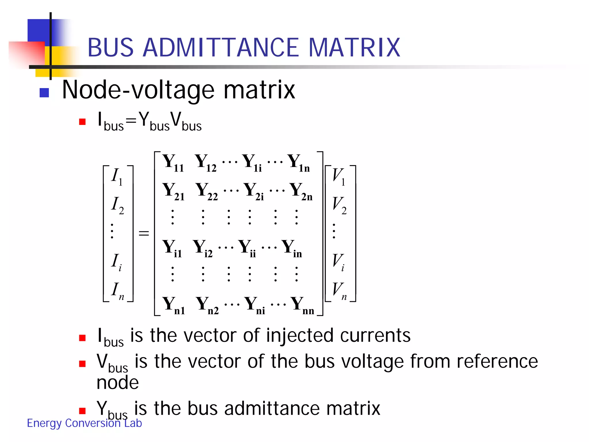
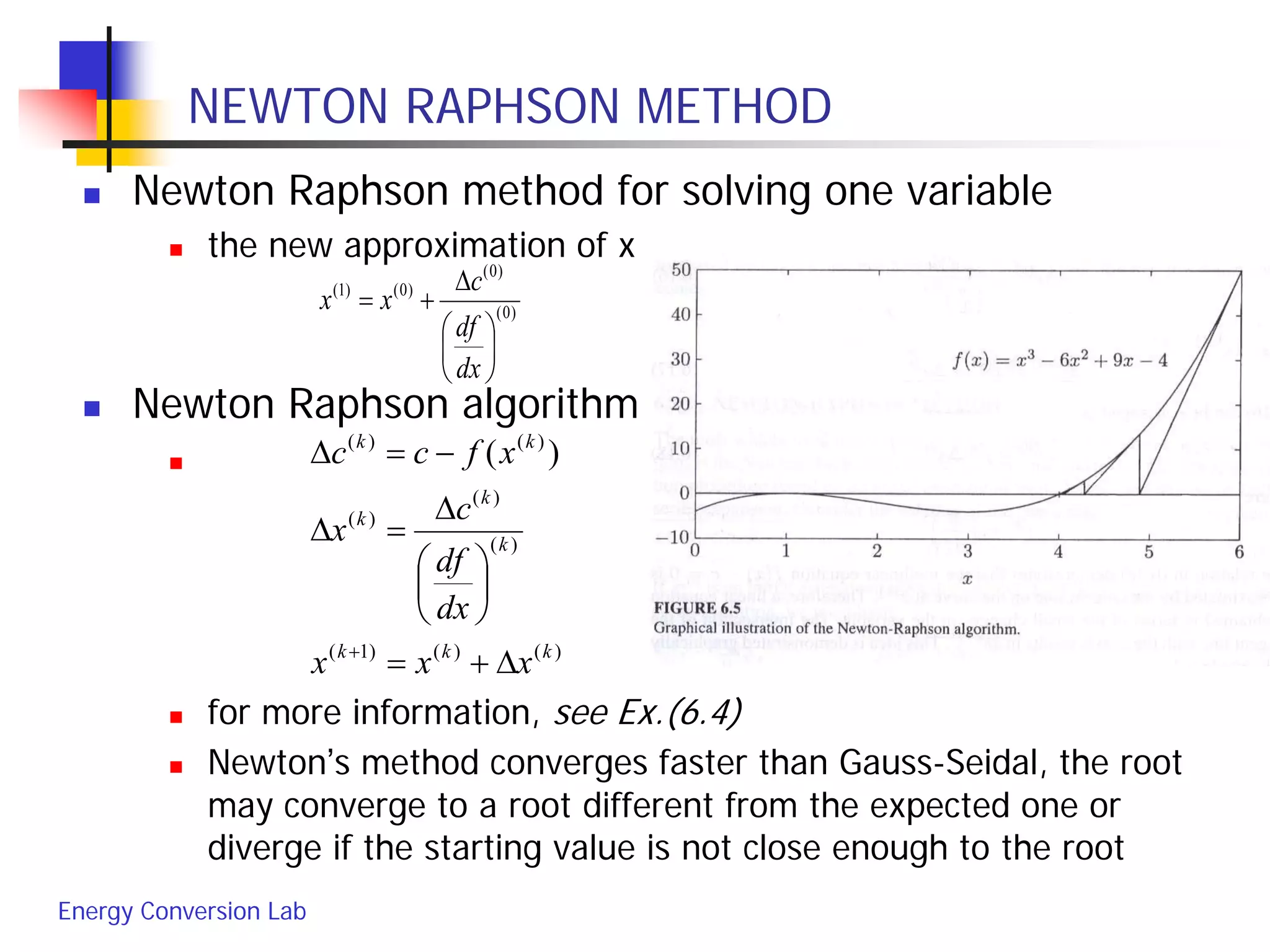
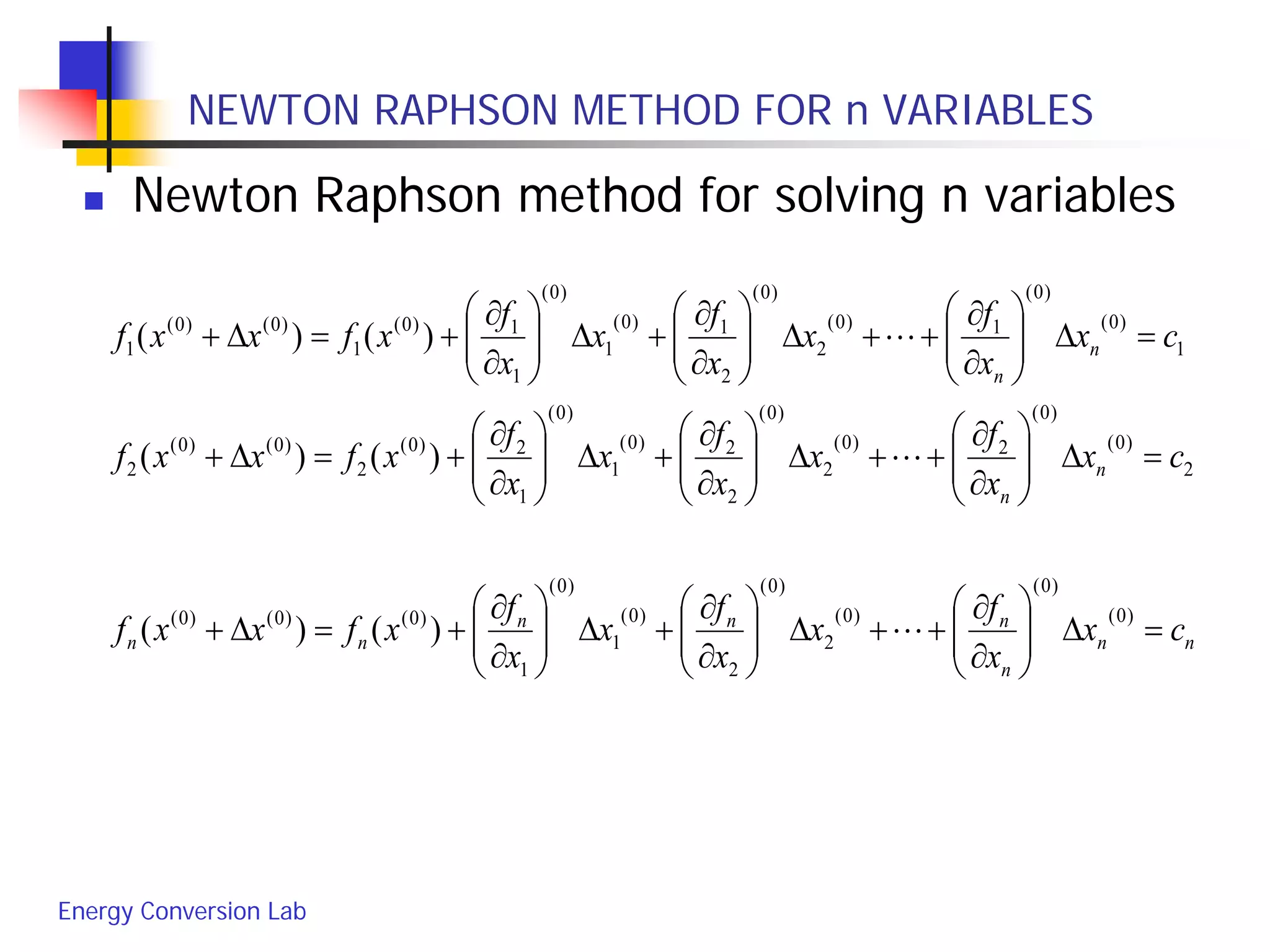
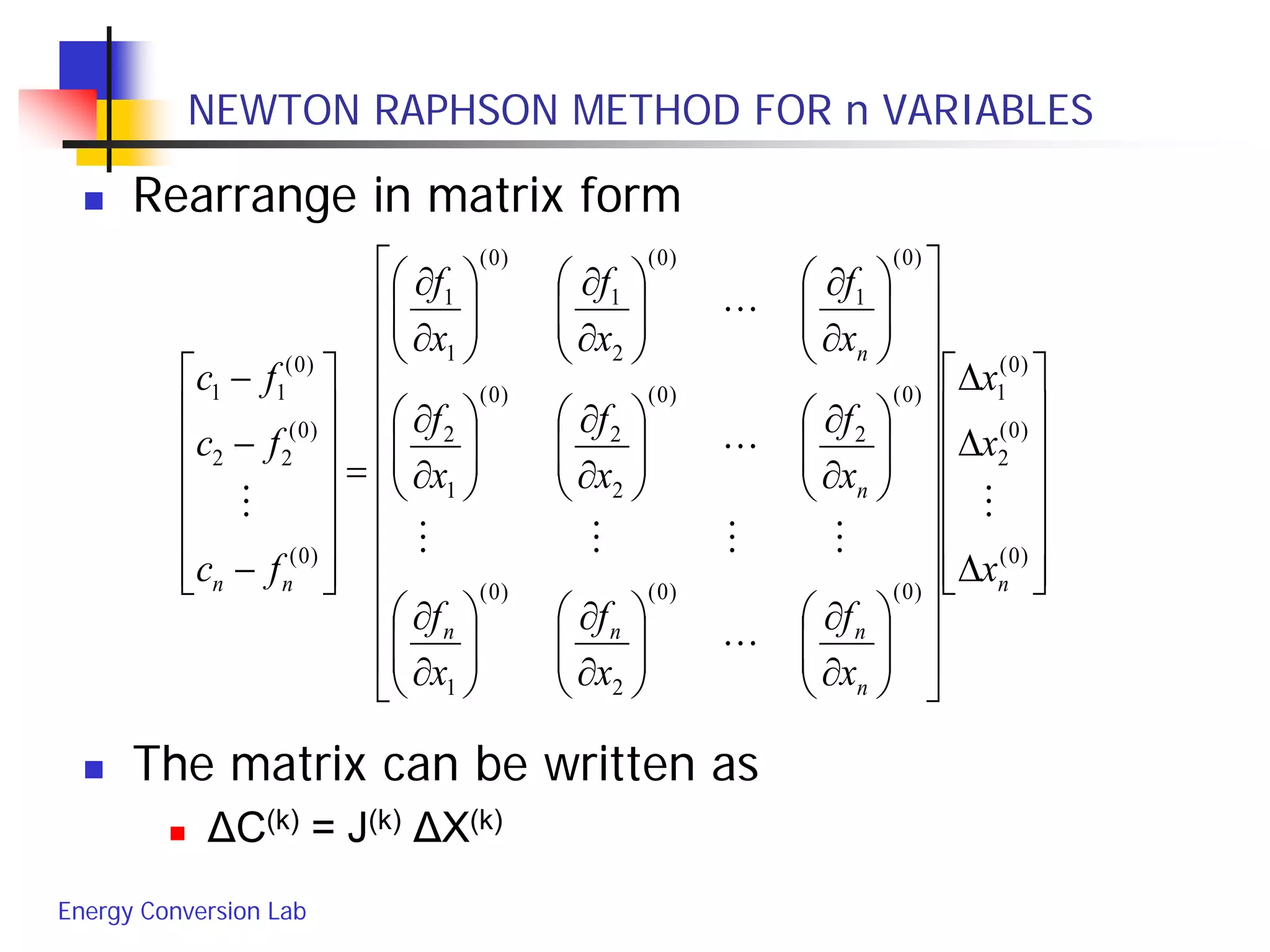
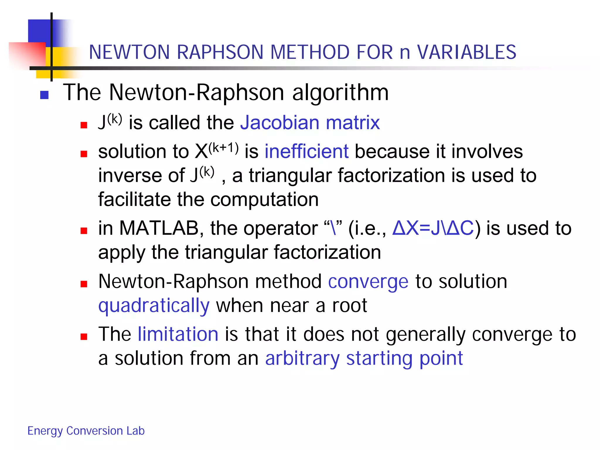
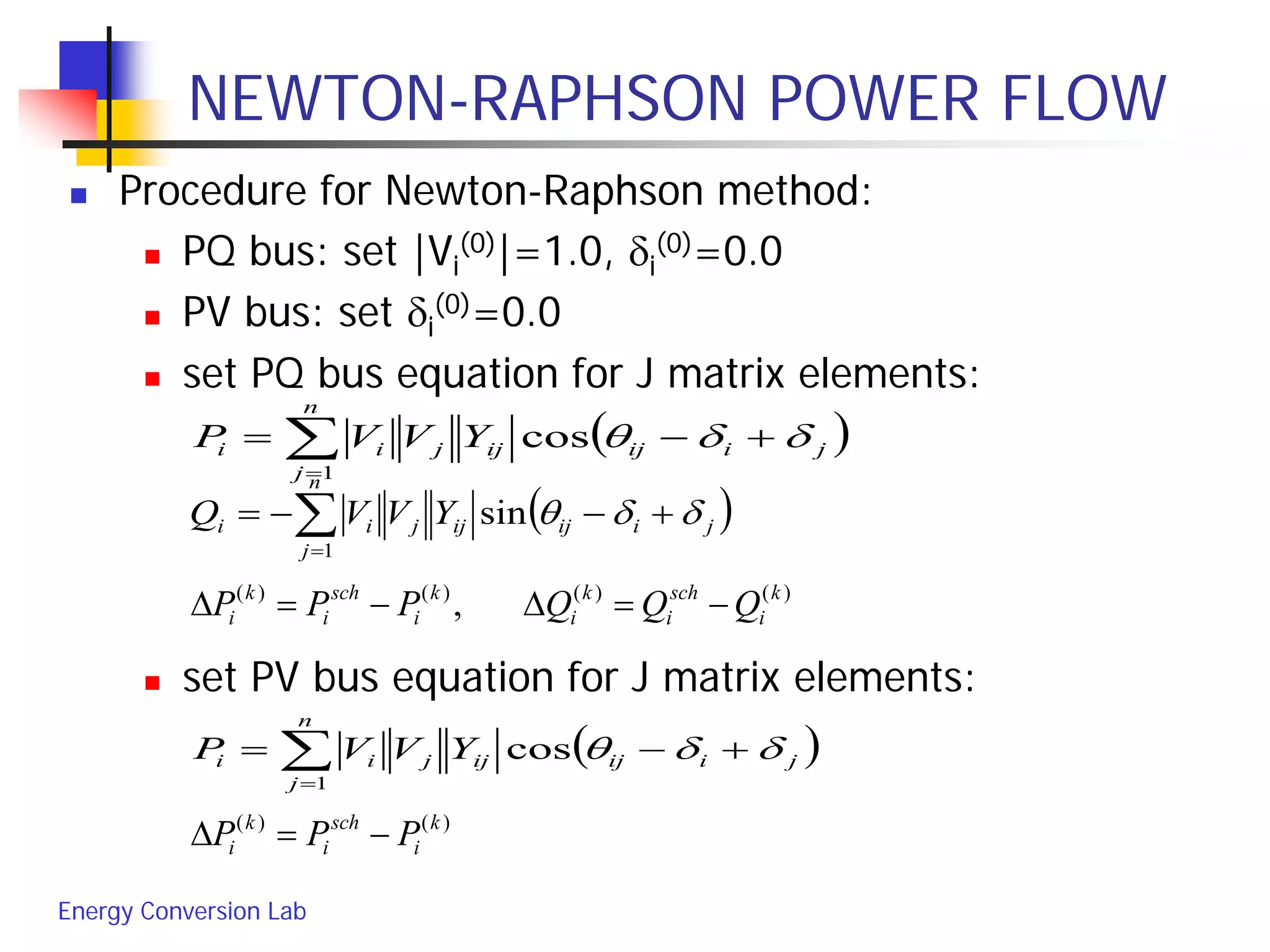
NEWTON RAPHSON METHOD FOR n VARIABLES
The Newton-Raphson algorithm for n-
dimensional case is
X(k+1) = X(k) +ΔX(k) = X(k) + [J(k)]-1ΔC(k)
where
−
−
−
=∆
)(
)(
22
)(
11
)(
k
nn
k
k
k
fc
fc
fc
C
∂
∂
∂
∂
∂
∂
∂
∂
∂
∂
∂
∂
∂
∂
∂
∂
∂
∂
=
)()(
2
)(
1
)(
2
)(
2
2
)(
1
2
)(
1
)(
2
1
)(
1
1
)(
k
n
n
k
n
k
n
k
n
kk
k
n
kk
k
x
f
x
f
x
f
x
f
x
f
x
f
x
f
x
f
x
f
J
∆
∆
∆
=∆
)(
)(
2
)(
1
)(
k
n
k
k
k
x
x
x
X
](https://image.slidesharecdn.com/apschap9powerflow-150705002455-lva1-app6891/75/APSA-LEC-9-24-2048.jpg)
![Energy Conversion Lab
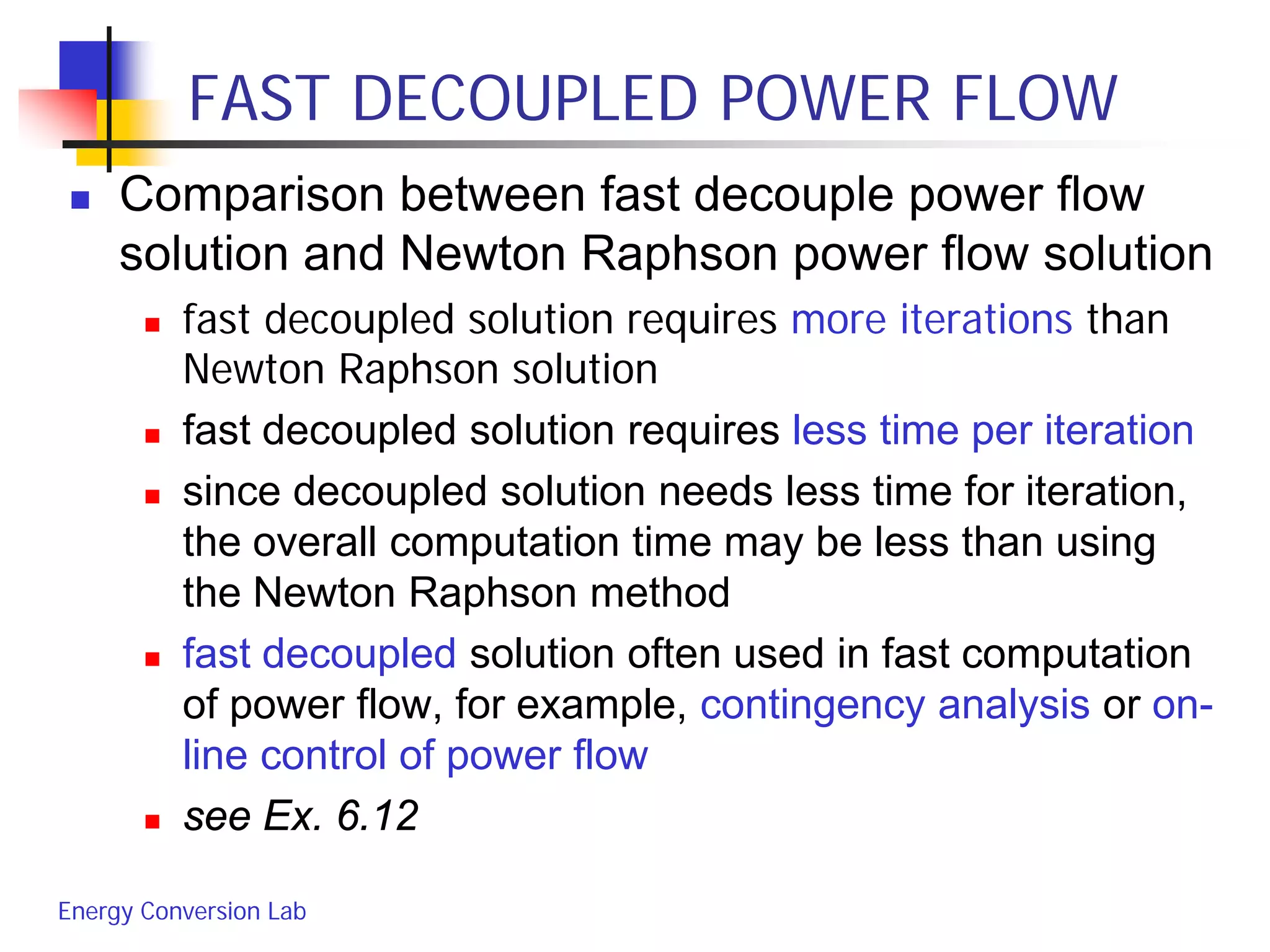
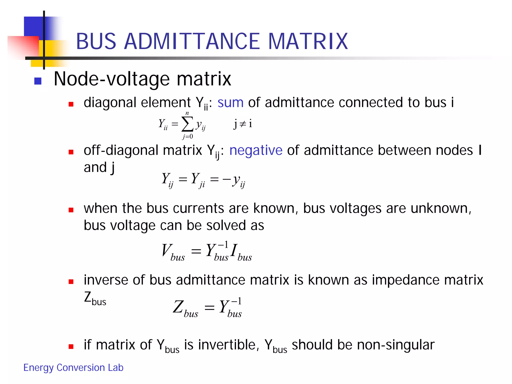
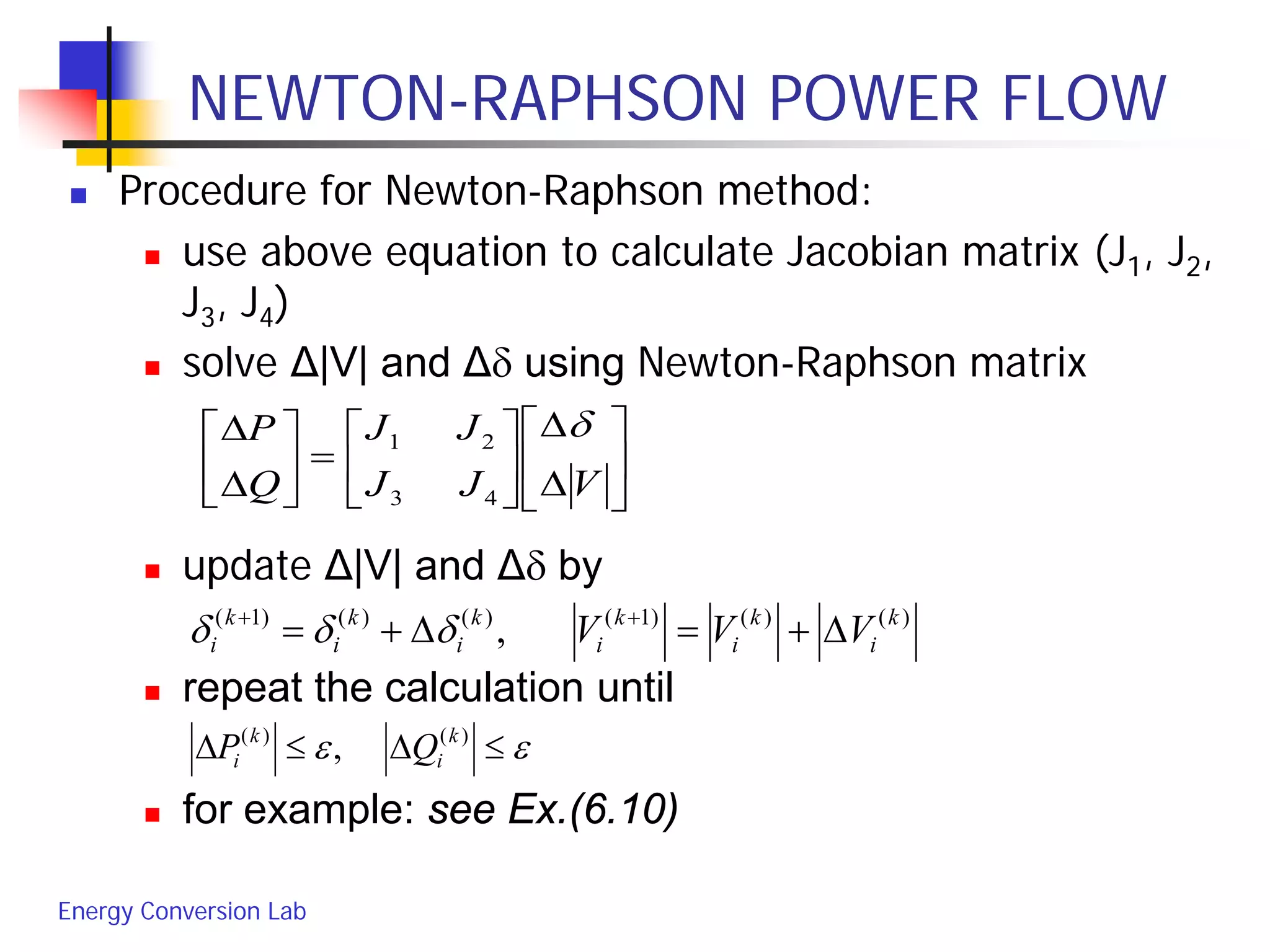
FAST DECOUPLED POWER FLOW
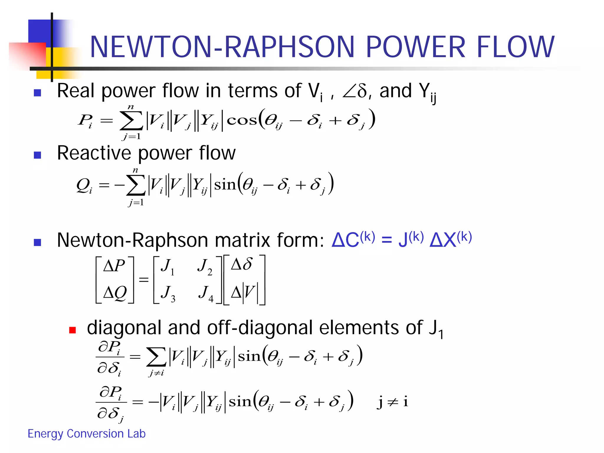
Consider the Newton-Raphson power flow equation
the power flow equation reduces to
ΔP = J1Δδ = [∂P/∂δ]Δδ, ΔQ = J4Δ|V| = [∂Q/∂|V|]Δ|V|
∂Pi/∂δi = -Qi - |Vi|2Bii, Bii = |Yii|sinθii is the imaginary part of the
diagonal elements
since Bii >> Qi, ∂Pi/∂δi (diagonal elements of J1) can be further
reduced to ∂Pi/∂δi = - |Vi|Bii (|Vi|2 ≈|Vi| )
off diagonal element of J1: ∂Pi/∂δi = - |Vi||Vj|Yijsin(θij-δi+δj), since δj-δi
is quite small, θij-δi+δj = θij, J1 = ∂Pi/∂δj = - |Vi||Vj|Bij
since |Vj|≈1, off diagonal elements of J1 = ∂Pi/∂δj = - |Vi|Bij
∆
∆
=
∆
∆
VJ
J
Q
P δ
4
1
0
0](https://image.slidesharecdn.com/apschap9powerflow-150705002455-lva1-app6891/75/APSA-LEC-9-33-2048.jpg)
![Energy Conversion Lab
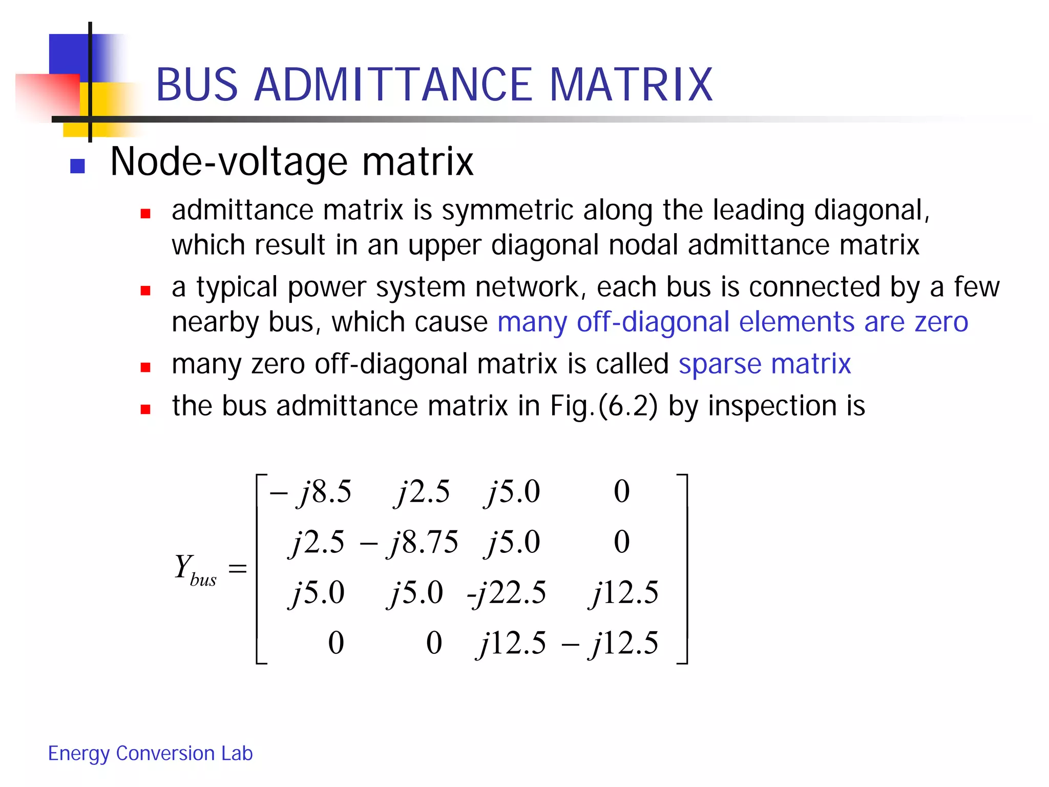
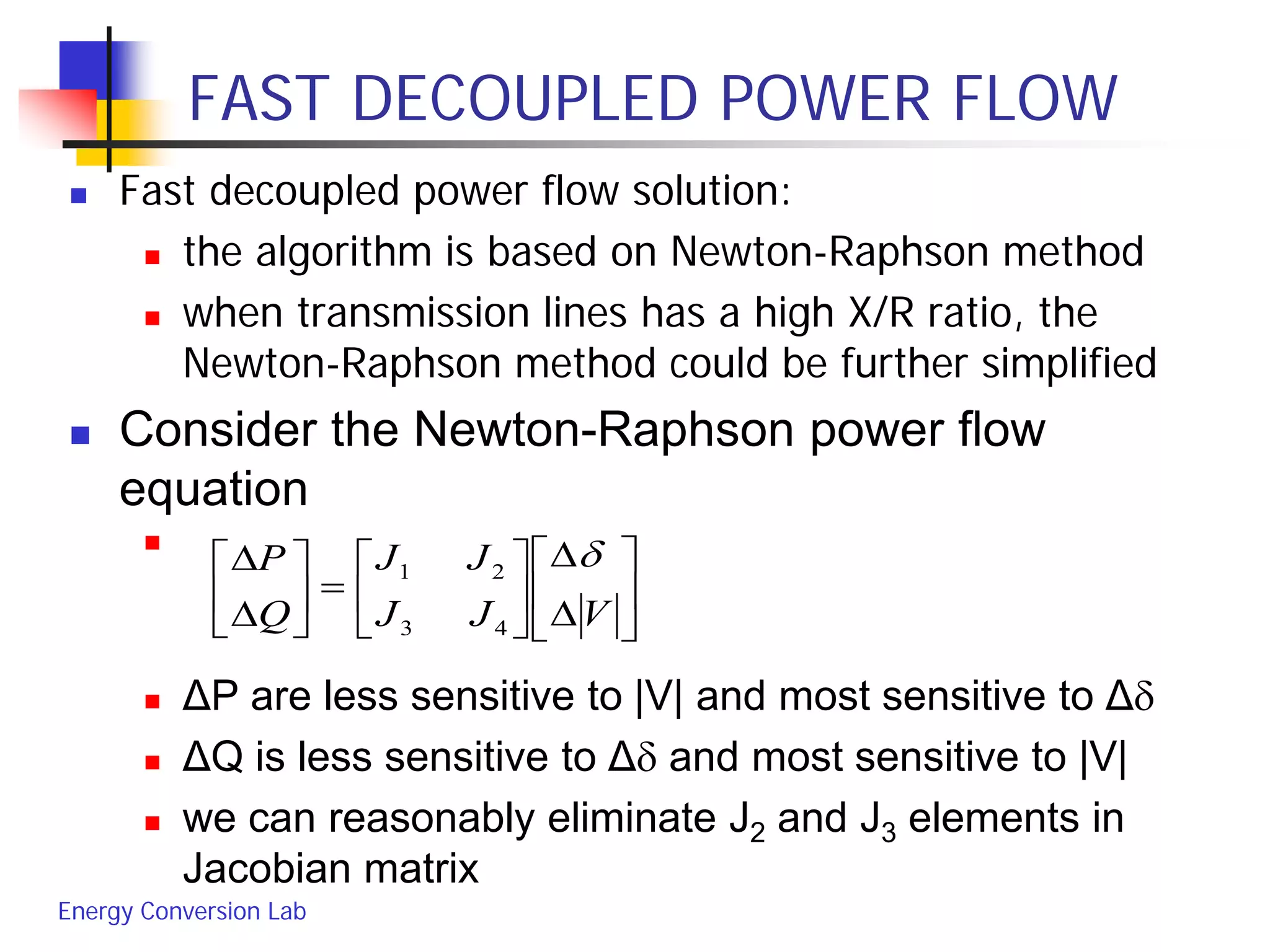
FAST DECOUPLED POWER FLOW
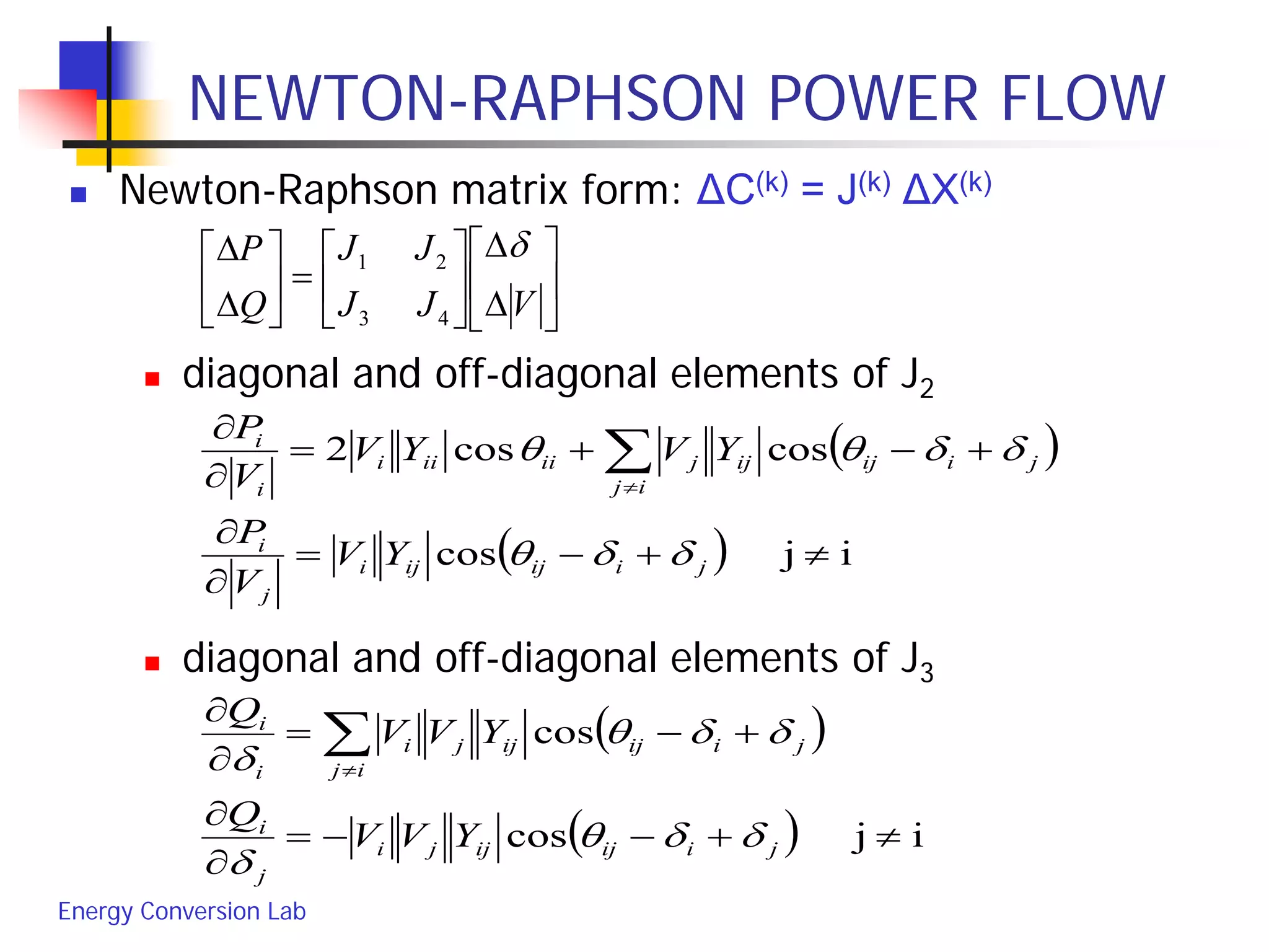
Consider the Newton-Raphson power flow
equation
similarly, diagonal elements of J4: ∂Qi/∂|Vi| = - |Vi|Bii
off diagonal elements of J4: ∂Qi/∂|Vj| = - |Vi|Bij
therefore, ΔP and ΔQ has the following forms
B’ and B” are the imaginary part of Ybus
the updated Δδ and Δ|V| can be obtained from
to calculate PQ bus, use simplified J1 and J4 to obtain
solution
to calculate PV bus, J4 can be further eliminated, only
J1 is used to obtain solution
VB
V
Q
B
V
P
ii
∆−=
∆
∆−=
∆ '''
,δ
[ ] [ ]
V
Q
BV
V
P
B
∆
−=∆
∆
−=∆
−− 11
",'δ](https://image.slidesharecdn.com/apschap9powerflow-150705002455-lva1-app6891/75/APSA-LEC-9-34-2048.jpg)