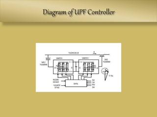
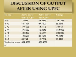
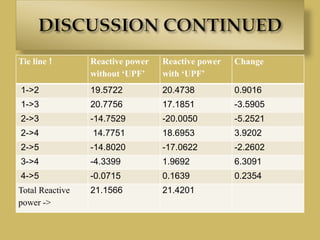
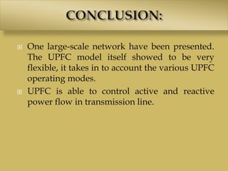
The document discusses optimal load flow control using the UPFC method, which enhances power transmission capacity and controls various parameters. It outlines the power flow analysis, the creation of the bus admittance matrix (Ybus), and employs the Newton-Raphson method for calculations. Additionally, it details the impact of UPFC on active and reactive power flow, along with its advantages for system stability and flexibility in power network design.

1. Presentation on
Optimal Load flow
control using UPFC
method

2.  The most common power system analysis tool
is the power flow (also known sometimes as
the load flow):
 power flow determines how the power flows in a
network
 also used to determine all bus voltages and all
currents,
 because of constant power models, power flow is a
nonlinear analysis technique,
 power flow is a steady-state analysis tool.

3.  First step in solving the power flow is to create what is
known as the bus admittance matrix, often called the
Ybus.
 The Ybus gives the relationships between all the bus
current injections, I, and all the bus voltages, V, I =
Ybus V
 The Ybus is developed by applying KCL at each bus in
the system to relate the bus current injections, the bus
voltages, and the branch impedances and admittances.

4. Determine the bus admittance matrix for the
network shown below.

5. 
| From | To | R | X | B/2 |
1 2 0.02 0.06 0.06;
1 3 0.08 0.24 0.05;
2 3 0.06 0.18 0.04;
2 4 0.06 0.18 0.04;
2 5 0.04 0.12 0.03;
3 4 0.01 0.03 0.02;
4 5 0.08 0.24 0.05];

6.  This method enables us to define the values of the
currents , the active and reactive powers, the active and
reactive power losses, and the power-factor of the
electrical supply network for different loads. It also
enables us to determine the degree of stability of the
network.

7.  flow chart newton rapson method.docx

8.  programme_5busstart.m
 programme_5busybus.m
 programme_5busjacobian.m
 programme_5busnewt.m

9. * *
1 1
1
1
1
( )
(cos sin )( )
Resolving into the real and imaginary parts
( cos sin )
( sin cos
ik
n n
j
i i i i ik k i k ik ik
k k
n
i k ik ik ik ik
k
n
i i k ik ik ik ik Gi Di
k
n
i i k ik ik ik i
k
S P jQ V Y V V V e G jB
V V j G jB
P V V G B P P
Q V V G B

 
 
 
 



    
  
   
 
 


 )k Gi DiQ Q 

10. o UPFC is a FACTS device which enhance power
transmission capacity.
o able to control all parameters of power
transmission(voltage, impedance, and phase
angle).
o UPF provides a consistent format to specify
power design .

12.  programme_5busupf.m

13. Tie line ! Active power
without ‘UPF’
Active power
with ‘UPF’
Change
1->2 77.9650 48.8279 -29.1326
1->3 74.1491 97.7007 23.5516
2->3 47.6626 14.1116 -33.551
2->4 47.3599 15.3646 -31.9953
2->5 44.8060 16.5174 -28.2886
3->4 12.0563 89.1578 77.1015
4->5 0.6754 19.7202 19.0448
Total active power
->
304.6698 301.4002

14. Tie line ! Reactive power
without ‘UPF’
Reactive power
with ‘UPF’
Change
1->2 19.5722 20.4738 0.9016
1->3 20.7756 17.1851 -3.5905
2->3 -14.7529 -20.0050 -5.2521
2->4 14.7751 18.6953 3.9202
2->5 -14.8020 -17.0622 -2.2602
3->4 -4.3399 1.9692 6.3091
4->5 -0.0715 0.1639 0.2354
Total Reactive
power ->
21.1566 21.4201

15.  Control of power flow
 Reduce reactive power flows, thus allowing the
lines to carry more active power.
 Increase the loading capability to their thermal
capabilities.
 Increase the system security through raising
transient stability limit.
 Provide greater flexibility in siting new
generation.

16.  One large-scale network have been presented.
The UPFC model itself showed to be very
flexible, it takes in to account the various UPFC
operating modes.
 UPFC is able to control active and reactive
power flow in transmission line.

17.  FACTS Modelling and simulation in Power networks,
Enrique Acha.
 ELECTRICAL POWER SYSTEM (FIFTH EDITION), C.
L. WADHWA.
 POWER SYSTEM ENGINEERING (SECOND
EDITION) , D. P. KOTHARI & I.J NAGRATH
 IEEE 100, The Authoritative Dictionary of IEEE Standards
Terms, Seventh Edition. New York: Institute of Electrical
and Electronics Engineers, Inc.