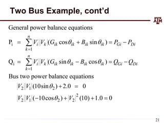
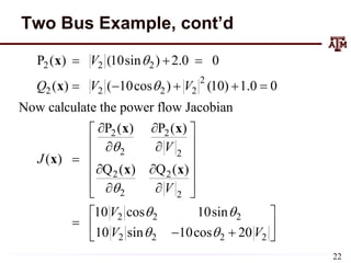
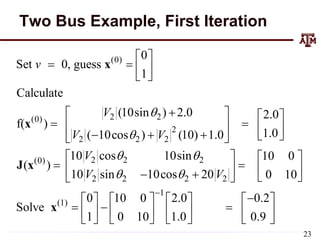
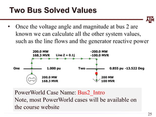
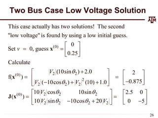
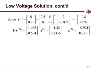
This document provides a summary of a lecture on power flow analysis. It begins with announcements about homework and reading assignments. It then discusses using the bus admittance matrix (Ybus) to solve for bus voltages and currents if one or the other is known. The remainder of the document discusses using the power balance equations and Newton-Raphson method to solve the power flow problem when bus real and reactive powers are known rather than voltages and currents. It provides examples of calculating the Jacobian matrix and using Newton-Raphson on a two bus system.

1. ECEN 615
Methods of Electric Power
Systems Analysis
Lecture 4: Power Flow
Prof. Tom Overbye
Dept. of Electrical and Computer Engineering
Texas A&M University
overbye@tamu.edu

2. Announcements
• Start reading Chapters 1 to 3 from the book (mostly
background material)
• Homework 1 is assigned today. It is due on
Thursday September 3
• Public website is
• https://overbye.engr.tamu.edu/ecen-615-fall-2020/
1

3. Using the Ybus
1
bus
If the voltages are known then we can solve for
the current injections:
If the current injections are known then we can
solve for the voltages:
where is the bus impedance matr
bus
bus bus


 
Y V I
Y I V Z I
Z ix
However, this requires that Ybus not be singular; note it will be
singular if there are no shunt connections!
2

4. Solving for Bus Currents
*
1 1 1
For example, in previous case assume
1.0
0.8 0.2
Then
12 15.9 12 16 1.0 5.60 0.70
12 16 12 15.9 0.8 0.2 5.58 0.88
Therefore the power injected at bus 1 is
S 1.0 (5.60
j
j j j
j j j j
V I
 
  

 
   
    

    
     
    
  
V
*
2 2 2
0.70) 5.60 0.70
(0.8 0.2) ( 5.58 0.88) 4.64 0.41
j j
S V I j j j
  
        
3

5. Solving for Bus Voltages
1
*
1 1 1
For example, in previous case assume
5.0
4.8
Then
12 15.9 12 16 5.0 0.0738 0.902
12 16 12 15.9 4.8 0.0738 1.098
Therefore the power injected is
S (0.0738 0.902) 5 0
j j j
j j j
V I j

 
  

 
   
     

     
     
     
    
I
*
2 2 2
.37 4.51
( 0.0738 1.098) ( 4.8) 0.35 5.27
j
S V I j j

       
4

6. Power Flow Analysis
• When analyzing power systems we know neither the
complex bus voltages nor the complex current
injections
• Rather, we know the complex power being consumed
by the load, and the power being injected by the
generators plus their voltage magnitudes
• Therefore we can not directly use the Ybus equations,
but rather must use the power balance equations
5

7. Power Balance Equations
1
bus
1
From KCL we know at each bus i in an n bus system
the current injection, , must be equal to the current
that flows into the network
Since = we also know
i
n
i Gi Di ik
k
n
i Gi Di ik k
k
I
I I I I
I I I Y V


  
  


I Y V
*
i
The network power injection is then S i i
V I

6

8. Power Balance Equations, cont’d
*
* * *
i
1 1
S
This is an equation with complex numbers.
Sometimes we would like an equivalent set of real
power equations. These can be derived by defining
n n
i i i ik k i ik k
k k
ik ik ik
i
V I V Y V V Y V
Y G jB
V
 
 
  
 
 
 

 
j
Recall e cos sin
i
j
i i i
ik i k
V e V
j



  
 
 
 
 
7

9. Real Power Balance Equations
* *
i
1 1
1
i
1
i
1
S ( )
(cos sin )( )
Resolving into the real and imaginary parts
P ( cos sin )
Q ( sin cos
ik
n n
j
i i i ik k i k ik ik
k k
n
i k ik ik ik ik
k
n
i k ik ik ik ik Gi Di
k
n
i k ik ik ik i
k
P jQ V Y V V V e G jB
V V j G jB
V V G B P P
V V G B

 
 
 
 



    
  
   
 
 


 )
k Gi Di
Q Q
 
8

10. Power Flow Analysis
• When analyzing power systems we know neither the
complex bus voltages nor the complex current
injections
• Rather, we know the complex power being consumed
by the load, and the power being injected by the
generators plus their voltage magnitudes
• Therefore we can not directly use the Ybus equations,
but rather must use the power balance equations
9

11. Power Flow Analysis
• Classic paper for this lecture is W.F. Tinney and C.E.
Hart, “Power Flow Solution by Newton’s Method,”
IEEE Power App System, Nov 1967
• Basic power flow is also covered in essentially any
power system analysis textbooks.
• We use the term “power flow” not “load flow” since
power flows not load. Also, the power flow usage is
not new (see title of Tinney’s 1967 paper, and note
Tinney references Ward’s 1956 power flow paper)
– A nice history of the power flow is given in an insert by
Alvarado and Thomas in T.J. Overbye, J.D. Weber,
“Visualizing the Electric Grid,” IEEE Spectrum, Feb 2001.
10

12. Early Power Flow System Size
• In 1957 Bill Tinney, in a paper titled “Digital Solutions
for Large Power Networks,” studied a 100 bus, 200
branch system (with 2 KB of memory)!
• In Tinney’s 1963 “Techniques for Exploiting Sparsity of
the Network Admittance Matrix” paper (which gave us
the Tinney Schemes 1, 2, and 3), uses 32 kB for 1000
nodes.
• In Tinney’s classic 1967 “Power Flow Solution by
Newton’s Method” paper he applies his method to
systems with up to about 1000 buses (with 32 kB of
memory) and provides a solution time of 51 seconds for
a 487 bus system.
11

13. Slack Bus
• We can not arbitrarily specify S at all buses because
total generation must equal total load + total losses
• We also need an angle reference bus.
• To solve these problems we define one bus as the
"slack" bus. This bus has a fixed voltage magnitude
and angle, and a varying real/reactive power injection.
• In an actual power system the slack bus does not really
exist; frequency changes locally when the power
supplied does not match the power consumed
12

14. Three Types of Power Flow Buses
• There are three main types of power flow buses
– Load (PQ) at which P/Q are fixed; iteration solves for voltage
magnitude and angle.
– Slack at which the voltage magnitude and angle are fixed;
iteration solves for P/Q injections
– Generator (PV) at which P and |V| are fixed; iteration solves
for voltage angle and Q injection
13

15. Newton-Raphson Algorithm
• Most common technique for solving the power
flow problem is to use the Newton-Raphson
algorithm
• Key idea behind Newton-Raphson is to use
sequential linearization
General form of problem: Find an such that
( ) 0
ˆ 
x
f x
14

16. Newton-Raphson Power Flow
i
1
In the Newton-Raphson power flow we use Newton's
method to determine the voltage magnitude and angle
at each bus in the power system.
We need to solve the power balance equations
P ( cos
n
i k ik ik
k
V V G 

 

i
1
sin )
Q ( sin cos )
ik ik Gi Di
n
i k ik ik ik ik Gi Di
k
B P P
V V G B Q Q

 

 
   

15

17. Power Flow Variables
2 2 2
n
2
Assume the slack bus is the first bus (with a fixed
voltage angle/magnitude). We then need to determine
the voltage angle/magnitude at the other buses.
( )
( )
G
n
P P
V
V


 
 
 
 
 
 
 
 
 
 
 
x
x f x
2
2 2 2
( )
( )
( )
D
n Gn Dn
G D
n Gn Dn
P
P P P
Q Q Q
Q Q Q
 
 
 
 
 
 
 
 
 
 
 
 
x
x
x
16

18. N-R Power Flow Solution
( )
( )
( 1) ( ) ( ) 1 ( )
The power flow is solved using the same procedure
discussed with the general Newton-Raphson:
Set 0; make an initial guess of ,
While ( ) Do
( ) ( )
1
End While
v
v
v v v v
v
v v

 


 
 
x x
f x
x x J x f x
17

19. Power Flow Jacobian Matrix
1 1 1
1 2
2 2 2
1 2
1 2
The most difficult part of the algorithm is determining
and inverting the n by n Jacobian matrix, ( )
( ) ( ) ( )
( ) ( ) ( )
( )
( ) ( ) ( )
n
n
n n n
n
f f f
x x x
f f f
x x x
f f f
x x x
  

   

  

   

  
  

J x
x x x
x x x
J x
x x x





 
 
 
 

18

20. Power Flow Jacobian Matrix, cont’d
i
i
i
1
Jacobian elements are calculated by differentiating
each function, f ( ), with respect to each variable.
For example, if f ( ) is the bus i real power equation
f ( ) ( cos sin )
n
i k ik ik ik ik Gi
k
x V V G B P P
 

   

x
x
i
1
i
f ( )
( sin cos )
f ( )
( sin cos ) ( )
Di
n
i k ik ik ik ik
i k
k i
i j ik ik ik ik
j
x
V V G B
x
V V G B j i
 

 




  


  


19

21. Two Bus Newton-Raphson Example
• For the two bus power system shown below, use
the Newton-Raphson power flow to determine the
voltage magnitude and angle at bus two. Assume
that bus one is the slack and SBase = 100 MVA.
Line Z = 0.1j
One Two
1.000 pu 1.000 pu
200 MW
100 MVR
0 MW
0 MVR
2
2
10 10
10 10
bus
j j
V j j
 
   
 
   

 
 
x Y
20

22. Two Bus Example, cont’d
i
1
i
1
2 1 2
2
2 1 2 2
General power balance equations
P ( cos sin )
Q ( sin cos )
Bus two power balance equations
(10sin ) 2.0 0
( 10cos ) (10) 1.0 0
n
i k ik ik ik ik Gi Di
k
n
i k ik ik ik ik Gi Di
k
V V G B P P
V V G B Q Q
V V
V V V
 
 




   
   
 
   


21

23. Two Bus Example, cont’d
2 2 2
2
2 2 2 2
2 2
2 2
2 2
2 2
2 2 2
2 2 2 2
P ( ) (10sin ) 2.0 0
( ) ( 10cos ) (10) 1.0 0
Now calculate the power flow Jacobian
P ( ) P ( )
( )
Q ( ) Q ( )
10 cos 10sin
10 sin 10cos 20
V
Q V V
V
J
V
V
V V




 
 
  
    
 
 
 
 
 

 
 
 
 
 
 
  
 
 
x
x
x x
x
x x
22

24. Two Bus Example, First Iteration
(0)
2 2
(0)
2
2 2 2
2 2 2
(0)
2 2 2 2
(1)
0
Set 0, guess
1
Calculate
(10sin ) 2.0 2.0
f( )
1.0
( 10cos ) (10) 1.0
10 cos 10sin 10 0
( )
10 sin 10cos 20 0 10
0 10 0
Solve
1 0 10
v
V
V V
V
V V


 
 
 
   
 

   
 
   
    
 
 
   
 
   
   
 
  
 
 
  
x
x
J x
x
1
2.0 0.2
1.0 0.9


    

     
    
23

25. Two Bus Example, Next Iterations
(1)
2
(1)
1
(2)
0.9(10sin( 0.2)) 2.0 0.212
f( )
0.279
0.9( 10cos( 0.2)) 0.9 10 1.0
8.82 1.986
( )
1.788 8.199
0.2 8.82 1.986 0.212 0.233
0.9 1.788 8.199 0.279 0.8586
f(

 
   
 
   
      
 

 
  

 
  
       
  
       

       
x
J x
x
(2) (3)
(3)
2
0.0145 0.236
)
0.0190 0.8554
0.0000906
f( ) Done! V 0.8554 13.52
0.0001175

   
 
   
   
 
    
 
 
x x
x
24

26. Two Bus Solved Values
• Once the voltage angle and magnitude at bus 2 are
known we can calculate all the other system values,
such as the line flows and the generator reactive power
output
Line Z = 0.1j
One Two
1.000 pu 0.855 pu
200 MW
100 MVR
200.0 MW
168.3 MVR
-13.522 Deg
200.0 MW
168.3 MVR
-200.0 MW
-100.0 MVR
PowerWorld Case Name: Bus2_Intro
Note, most PowerWorld cases will be available on
the course website
25

27. Two Bus Case Low Voltage Solution
(0)
2 2
(0)
2
2 2 2
This case actually has two solutions! The second
"low voltage" is found by using a low initial guess.
0
Set 0, guess
0.25
Calculate
(10sin ) 2.0
f( )
( 10cos ) (10) 1.0
v
V
V V


 
   
 

 
  
  
 
 
x
x
2 2 2
(0)
2 2 2 2
2
0.875
10 cos 10sin 2.5 0
( )
10 sin 10cos 20 0 5
V
V V
 
 
 
  

 
   
 
   
  
 
 
J x
26

28. Low Voltage Solution, cont'd
1
(1)
(2) (2) (3)
0 2.5 0 2 0.8
Solve
0.25 0 5 0.875 0.075
1.462 1.42 0.921
( )
0.534 0.2336 0.220


       
  
       
 
       
 
     
  
     
     
x
f x x x
27

29. Practical Power Flow Software Note
• Most commercial software packages have built in
defaults to prevent convergence to low voltage
solutions.
– One approach is to automatically change the load model from
constant power to constant current or constant impedance
when the load bus voltage gets too low
– In PowerWorld these defaults can be modified on the Tools,
Simulator Options, Advanced Options page; note you also
need to disable the “Initialize from Flat Start Values” option
– The PowerWorld case Bus2_Intro_Low is set solved to the
low voltage solution
– Initial bus voltages can be set using the Bus Information
Dialog
28

30. Two Bus Region of Convergence
Slide shows the region of convergence for different initial
guesses of bus 2 angle (x-axis) and magnitude (y-axis)
Red region
converges
to the high
voltage
solution,
while the
yellow region
converges
to the low
voltage
solution
29

31. Power Flow Fractal Region of
Convergence
• Earliest paper showing fractal power flow regions of
convergence is by C.L DeMarco and T.J. Overbye,
“Low Voltage Power Flow Solutions and Their Role
in Exit Time Bases Security Measures for Voltage
Collapse,” Proc. 27th IEEE CDC, December 1988
• A more widely known paper is J.S. Thorp, S.A.
Naqavi, “Load-Flow Fractals Draw Clues to Erratic
Behavior,” IEEE Computer Applications in Power,
January 1997
30

32. PV Buses
• Since the voltage magnitude at PV buses is fixed
there is no need to explicitly include these voltages
in x or write the reactive power balance equations
– the reactive power output of the generator varies to
maintain the fixed terminal voltage (within limits)
– optionally these variations/equations can be included by
just writing the explicit voltage constraint for the
generator bus
|Vi | – Vi setpoint = 0
31

33. Three Bus PV Case Example
Line Z = 0.1j
Line Z = 0.1j Line Z = 0.1j
One Two
1.000 pu
0.941 pu
200 MW
100 MVR
170.0 MW
68.2 MVR
-7.469 Deg
Three 1.000 pu
30 MW
63 MVR
2 2 2 2
3 3 3 3
2 2 2
For this three bus case we have
( )
( ) ( ) 0
V ( )
G D
G D
D
P P P
P P P
Q Q


 
   
   
    
   

   
 
 
x
x f x x
x
32

34. Modeling Voltage Dependent Load
So far we've assumed that the load is independent of
the bus voltage (i.e., constant power). However, the
power flow can be easily extended to include voltage
depedence with both the real and reactive l
Di Di
1
1
oad. This
is done by making P and Q a function of :
( cos sin ) ( ) 0
( sin cos ) ( ) 0
i
n
i k ik ik ik ik Gi Di i
k
n
i k ik ik ik ik Gi Di i
k
V
V V G B P P V
V V G B Q Q V
 
 


   
   


33

35. Voltage Dependent Load Example
2
2 2 2 2
2 2
2 2 2 2 2
2 2 2 2
In previous two bus example now assume the load is
constant impedance, so
P ( ) (10sin ) 2.0 0
( ) ( 10cos ) (10) 1.0 0
Now calculate the power flow Jacobian
10 cos 10sin 4.0
( )
10
V V
Q V V V
V V
J


 
  
    


x
x
x
2 2 2 2 2
sin 10cos 20 2.0
V V V
 
 
 
  
 
34

36. Voltage Dependent Load, cont'd
(0)
2
2 2 2
(0)
2 2
2 2 2 2
(0)
1
(1)
0
Again set 0, guess
1
Calculate
(10sin ) 2.0 2.0
f( )
1.0
( 10cos ) (10) 1.0
10 4
( )
0 12
0 10 4 2.0 0.1667
Solve
1 0 12 1.0 0.9167
v
V V
V V V



 
   
 
 
  
 
   
 
 
  
 
 
  
 

      
  
     
     
x
x
J x
x

 
 
35

37. Voltage Dependent Load, cont'd
Line Z = 0.1j
One Two
1.000 pu
0.894 pu
160 MW
80 MVR
160.0 MW
120.0 MVR
-10.304 Deg
160.0 MW
120.0 MVR
-160.0 MW
-80.0 MVR
With constant impedance load the MW/Mvar load at
bus 2 varies with the square of the bus 2 voltage
magnitude. This if the voltage level is less than 1.0,
the load is lower than 200/100 MW/Mvar
PowerWorld Case Name: Bus2_Intro_Z
36

38. Generator Reactive Power Limits
• The reactive power output of generators varies to
maintain the terminal voltage; on a real generator
this is done by the exciter
• To maintain higher voltages requires more
reactive power
• Generators have reactive power limits, which are
dependent upon the generator's MW output
• These limits must be considered during the power
flow solution.
37

39. Generator Reactive Limits, cont'd
• During the power flow once a solution is obtained
there is a check to make sure the generator reactive
power output is within its limits
• If the reactive power is outside of the limits, fix Q at
the max or min value, and resolve treating the
generator as a PQ bus
– this is know as "type-switching"
– also need to check if a PQ generator can again regulate
• Rule of thumb: to raise system voltage we need to
supply more vars
38

40. 400 MVA
15 kV
400 MVA
15/345 kV
T1
T2
800 MVA
345/15 kV
800 MVA
15 kV
520 MVA
80 MW
40 Mvar
280 Mvar 800 MW
Line 3
345 kV
Line
2
Line
1
345 kV
100 mi
345 kV
200 mi
50 mi
1 4 3
2
5
Single-line diagram
The N-R Power Flow: 5-bus Example
This five bus example is taken from Chapter 6 of Power
System Analysis and Design by Glover, Overbye, and Sarma,
6th Edition, 2016
39

41. Bus Type
V
per
unit

degrees
PG
per
unit
QG
per
unit
PL
per
unit
QL
per
unit
QGmax
per
unit
QGmin
per
unit
1 Swing 1.0 0   0 0  
2 Load   0 0 8.0 2.8  
3 Constant
voltage
1.05  5.2  0.8 0.4 4.0 -2.8
4 Load   0 0 0 0  
5 Load   0 0 0 0  
Table 1.
Bus input
data
Bus-to-
Bus
R’
per unit
X’
per unit
G’
per unit
B’
per unit
Maximum
MVA
per unit
2-4 0.0090 0.100 0 1.72 12.0
2-5 0.0045 0.050 0 0.88 12.0
4-5 0.00225 0.025 0 0.44 12.0
Table 2.
Line input data
The N-R Power Flow: 5-bus Example
40

42. Bus-to-
Bus
R
per
unit
X
per
unit
Gc
per
unit
Bm
per
unit
Maximum
MVA
per unit
Maximum
TAP
Setting
per unit
1-5 0.00150 0.02 0 0 6.0 —
3-4 0.00075 0.01 0 0 10.0 —
Table 3.
Transformer
input data
Bus Input Data Unknowns
1 V1 = 1.0, 1 = 0 P1, Q1
2 P2 = PG2-PL2 = -8
Q2 = QG2-QL2 = -2.8
V2, 2
3 V3 = 1.05
P3 = PG3-PL3 = 4.4
Q3, 3
4 P4 = 0, Q4 = 0 V4, 4
5 P5 = 0, Q5 = 0 V5, 5
Table 4. Input data
and unknowns
The N-R Power Flow: 5-bus Example
41

43. Five Bus Case Ybus
PowerWorld Case Name: GOS_FiveBus

44. Ybus Calculation Details
0
23
21 
 Y
Y
unit
per
j
j
jX
R
Y 91964
.
9
89276
.
0
1
.
0
009
.
0
1
1
'
24
'
24
24 








unit
per
j
j
jX
R
Y 83932
.
19
78552
.
1
05
.
0
0045
.
0
1
1
'
25
'
25
25 








2
2
1
1 '
25
'
24
'
25
'
25
'
24
'
24
22
B
j
B
j
jX
R
jX
R
Y 





2
88
.
0
2
72
.
1
)
83932
.
19
78552
.
1
(
)
91964
.
9
89276
.
0
( j
j
j
j 





unit
per
j 




 624
.
84
5847
.
28
4590
.
28
67828
.
2
Elements of Ybus connected to bus 2
43

45. Initial Bus Mismatches
44

46. Initial Power Flow Jacobian
45

47. ]
)
0
(
)
0
(
cos[
){
0
(
)
(
)
0
( 21
1
2
1
21
2
2
2
2
2 

 





 V
Y
V
P
x
P
P
P
]
)
0
(
)
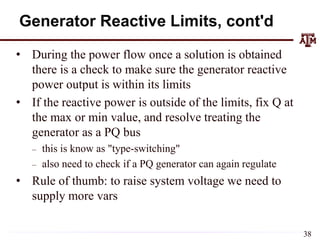
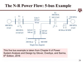
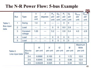
0
(
cos[
]
cos[ 23
3
2
3
23
22
2
22 


 



 V
Y
V
Y
]
)
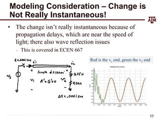
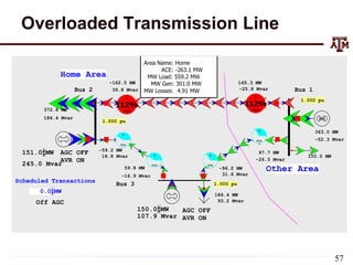
0
(
)
0
(
cos[ 24
4
2
4
24 

 

 V
Y
]}
)
0
(
)
0
(
cos[ 25
5
2
5
25 

 

 V
Y
)
624
.
84
cos(
)
0
.
1
(
5847
.
28
{
0
.
1
0
.
8 



)
143
.
95
cos(
)
0
.
1
(
95972
.
9 


)}
143
.
95
cos(
)
0
.
1
(
9159
.
19 


unit
per
99972
.
7
)
10
89
.
2
(
0
.
8 4






 
]
)
0
(
)
0
(
sin[
)
0
(
)
0
(
)
0
(
1 24
4
2
4
24
2
24 

 

 V
Y
V
J
]
143
.
95
sin[
)
0
.
1
)(
95972
.
9
)(
0
.
1
( 


unit
per
91964
.
9


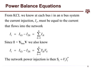
Hand Calculation Details
46

48. Five Bus Power System Solved
slack
One
Two
Three
Four
Five
A
MVA
A
MVA
A
MVA
A
MVA
A
MVA
1.000 pu 0.974 pu
0.834 pu
1.019 pu
1.050 pu
0.000 Deg -4.548 Deg
-22.406 Deg
-2.834 Deg
-0.597 Deg
395 MW
114 Mvar
520 MW
337 Mvar
800 MW
280 Mvar
80 MW
40 Mvar
47

49. 37 Bus Case Example
slack
Aggieland Power and Light
SLA CK345
SLA CK138
HOWDY345
HOWDY138
HOWDY69
12MA N69
GIGEM69
KYLE69
KYLE138
WEB138
WEB69
BONFIRE69
FISH69
RING69
T REE69
CENT URY69
REVEILLE69
T EXA S69
T EXA S138
T EXA S345
BA T T 69
NORT HGA T E69
MA ROON69
SPIRIT 69
YELL69
RELLIS69
WHIT E138
RELLIS138
BUSH69
MSC69
RUDDER69
HULLA BA LOO138
REED69
REED138
A GGIE138 A GGIE345
22%
A
MVA
23%
A
MVA
77%
A
MVA
40%
A
MVA
75%
A
MVA
78%
A
MVA
78%
A
MVA
17%
A
MVA
45%
A
MVA
81%
A
MVA
A
MVA
67%
A
MVA
28%
A
MVA
33%
A
MVA
38%
A
MVA
60%
A
MVA
60%
A
MVA
23%
A
MVA
23%
A
MVA
23%
A
MVA
A
MVA
58%
A
MVA
68%
A
MVA
68%
A
MVA
14%
A
MVA
82%
A
MVA
72%
A
MVA
40%
A
MVA
41%
A
MVA
34%
A
MVA
68%
A
MVA
68%
A
MVA
68%
A
MVA
35%
A
MVA
15%
A
MVA
19%
A
MVA
56%
A
MVA
66%
A
MVA
40%
A
MVA
70%
A
MVA
71%
A
MVA
71%
A
MVA
1.00 pu
0.96 pu
1.01 pu
1.03 pu
0.92 pu
0.91 pu
0.96 pu
0.94 pu
0.94 pu
0.94 pu
0.90 pu
0.94 pu
0.93 pu
0.99 pu
0.98 pu
1.00 pu
0.94 pu
0.94 pu
1.00 pu
0.992 pu
1.00 pu
0.98 pu
0.97 pu
0.95 pu
0.95 pu
0.93 pu
0.93 pu 0.93 pu
0.96 pu
0.95 pu
0.94 pu
1.00 pu
1.02 pu
73%
A
MVA
1.02 pu
74%
A
MVA
PLUM138
18%
A
MVA
0.99 pu
A
MVA
0.94 pu
39%
A
MVA
905 MW
34 MW
0 Mvar
59 MW
17 Mvar
MW
0
100 MW
30 Mvar
20 MW
8 Mvar
MW
200
100 MW
30 Mvar
61 MW
17 Mvar
59 MW
6 Mvar
69 MW
0 Mvar
93 MW
58 Mvar
58 MW
17 Mvar
MW
10
36 MW
24 Mvar
96 MW
20 Mvar
MW
45
37 MW
14 Mvar
53 MW
21 Mvar
0.0 Mvar 29 MW
8 Mvar
93 MW
65 Mvar
82 MW
27 Mvar
0.0 Mvar
35 MW
11 Mvar
25 MW
10 Mvar
38 MW
10 Mvar 22 MW
0 Mvar
0.0 Mvar
0.0 Mvar
0.0 Mvar
0.0 Mvar
0.0 Mvar
0.0 Mvar
MW
90
31 MW
13 Mvar
MW
50
27 MW
4 Mvar
MW
5
49 MW
17 Mvar
Total Losses: 44.40 MW
Total Load 1420.0 MW
MW
110
MW
50
deg
0
tap
1.0875
tap
1.0625
tap
1.0000
279.1 MW
124.4 MW
99%
A
MVA
86%
A
MVA
86%
A
MVA
128%
A
MVA
120%
A
MVA
107%
A
MVA
101%
A
MVA
101%
A
MVA
102%
A
MVA
PowerWorld Case Name: Aggieland37
48

50. Voltage Control Example: 37 Buses
slack
SLA CK345
SLA CK138
RA Y345
RA Y138
RA Y69
FERNA 69
A
MVA
DEMA R69
BLT 69
BLT 138
BOB138
BOB69
WOLEN69
SHIMKO69
ROGER69
UIUC69
PET E69
HISKY69
T IM69
T IM138
T IM345
PA I69
GROSS69
HA NNA H69
A MA NDA 69
HOMER69
LA UF69
MORO138
LA UF138
HA LE69
PA T T EN69
WEBER69
BUCKY138
SA VOY69
SA VOY138
JO138 JO345
A
MVA
A
MVA
A
MVA
A
MVA
A
MVA
A
MVA
A
MVA
A
MVA
A
MVA
A
MVA
A
MVA
A
MVA
A
MVA
A
MVA
A
MVA
A
MVA
A
MVA
A
MVA
A
MVA
A
MVA
A
MVA
A
MVA
A
MVA
A
MVA
A
MVA
A
MVA
A
MVA
A
MVA
A
MVA
A
MVA
A
MVA
A
MVA
A
MVA
A
MVA
A
MVA
A
MVA
A
MVA
A
MVA
A
MVA
A
MVA
A
MVA
A
MVA
A
MVA
A
MVA
A
MVA
A
MVA
A
MVA
A
MVA
A
MVA
A
MVA
1.03 pu
1.01 pu
1.02 pu
1.03 pu
1.01 pu
1.00 pu
1.00 pu
0.99 pu
1.02 pu
1.01 pu
1.00 pu
1.01 pu
1.01 pu
1.01 pu
1.01 pu
1.02 pu
1.00 pu
1.00 pu
1.02 pu
0.997 pu
0.99 pu
1.00 pu
1.02 pu
1.00 pu
1.01 pu
1.00 pu
1.00 pu 1.00 pu
1.01 pu
1.02 pu
1.02 pu
1.02 pu
1.03 pu
A
MVA
1.02 pu
A
MVA
A
MVA
LYNN138
A
MVA
1.02 pu
A
MVA
1.00 pu
A
MVA
219 MW
52 Mvar
21 MW
7 Mvar
45 MW
12 Mvar
MW
157
45 Mvar
37 MW
13 Mvar
12 MW
5 Mvar
MW
150
-0 Mvar
56 MW
13 Mvar
15 MW
5 Mvar
14 MW
2 Mvar
MW
38
3 Mvar
45 MW
0 Mvar
58 MW
36 Mvar
36 MW
10 Mvar
MW
0
0 Mvar
22 MW
15 Mvar
60 MW
12 Mvar
MW
20
9 Mvar
23 MW
6 Mvar
33 MW
13 Mvar
15.9 Mvar 18 MW
5 Mvar
58 MW
40 Mvar
51 MW
15 Mvar
14.3 Mvar
33 MW
10 Mvar
15 MW
3 Mvar
23 MW
6 Mvar 14 MW
3 Mvar
4.8 Mvar
7.2 Mvar
12.8 Mvar
29.0 Mvar
7.4 Mvar
20.8 Mvar
MW
92
10 Mvar
19 MW
8 Mvar
MW
150
-0 Mvar
17 MW
3 Mvar
MW
0
0 Mvar
14 MW
4 Mvar
pu
1.010
0.0 Mvar
System Losses: 11.51 MW
PowerWorld Case Name: Bus37_VoltageControl
49

51. Power System Operations Overview
• Goal is to provide an intuitive feel for power
system operation
• Emphasis will be on the impact of the transmission
system
• Introduce basic power flow concepts through small
system examples
50

52. Power System Basics
• All power systems have three major components:
Generation, Load and Transmission/Distribution.
• Generation: Creates electric power.
• Load: Consumes electric power.
• Transmission/Distribution: Transmits electric power
from generation to load.
– Lines/transformers operating at voltages above 100 kV are
usually called the transmission system. The transmission
system is usually networked.
– Lines/transformers operating at voltages below 100 kV are
usually called the distribution system (radial).
51

53. Large System Example: Texas 2000
Bus Synthetic System
This case requires the commercial version of PowerWorld
since the GOS Version is limited to 42 Buses
52

54. Three Bus PowerWorld Simulator Case
Bus 2 Bus 1
Bus 3
Home Area
Other Area
slack
Scheduled Transactions
1.00 pu
25.4 MW
5.3 Mvar
25.5 MW
-4.9 Mvar
34.3 MW
10.6 Mvar
34.5 MW
-10.0 Mvar
10.1 MW
-3.0 Mvar
10.1 MW
3.1 Mvar
1.00 pu
1.00 pu
A
MVA
A
MVA
A
MVA
A
MVA
A
MVA
A
MVA
MW
0.0
Off AGC
210.8 MW
105.4 Mvar
MW
151.0
MW
150.0
Mvar
39.7
Mvar
121.3
105.4 MW
52.7 Mvar
115.4 MW
-1.9 Mvar
100 MW
AGC OFF
AVR ON
AGC ON
AVR ON
ACE: -15.5 MW
Area Name: Home
MW Load: 316.2 MW
MW Losses: 0.28 MW
MW Gen: 301.0 MW
Load with
green
arrows
indicating
amount
of MW
flow
Used
to control
output of
generator
Note the
power
balance at
each bus
Direction of green arrow is used to indicate
direction of real power (MW) flow; the blue
arrows show the reactive power
PowerWorld Case Name: B3Slow
53

55. Basic Power Control
• Opening a circuit breaker causes the power flow to
instantaneously (nearly) change.
• No other way to directly control power flow in a
transmission line.
• By changing generation we can indirectly change this
flow.
• Power flow in transmission line is limited by heating
considerations
• Losses (I^2 R) can heat up the line, causing it to sag.
54

56. Modeling Consideration – Change is
Not Really Instantaneous!
• The change isn’t really instantaneous because of
propagation delays, which are near the speed of
light; there also wave reflection issues
– This is covered in ECEN 667
Red is the vs end, green the v2 end
55

57. Transmission Line Limits
• Power flow in transmission line is limited by heating
considerations.
• Losses (I2 R) can heat up the line, causing it to sag.
• Each line has a limit; many utilities use winter/summer
limits.
56

58. Overloaded Transmission Line
Bus 2 Bus 1
Bus 3
Home Area
Other Area
slack
Scheduled Transactions
1.000 pu
-162.5 MW
39.8 Mvar
165.3 MW
-25.8 Mvar
-59.2 MW
18.8 Mvar
59.8 MW
-16.9 Mvar
-96.2 MW
31.6 Mvar
97.7 MW
-26.5 Mvar
1.000 pu
1.000 pu
A
MVA
A
MVA
A
MVA
A
MVA
MW
0.0
Off AGC
372.8 MW
186.4 Mvar
MW
151.0
MW
150.0
107.9 Mvar
245.0 Mvar
186.4 MW
93.2 Mvar
363.0 MW
-52.3 Mvar
100.0 MW
AGC OFF
AVR ON
AGC OFF
AVR ON
ACE: -263.1 MW
Area Name: Home
MW Load: 559.2 MW
MW Losses: 4.91 MW
MW Gen: 301.0 MW
112%
A
MVA
112%
A
MVA
57

59. Interconnected Operation
Balancing Authority (BA) Areas
• North American Eastern and Western grids are divided
into balancing authority areas (BA)
– Often just called an area
• Transmission lines that join two areas are known as
tie-lines.
• The net power out of an area is the sum of the flow on
its tie-lines.
• The flow out of an area is equal to
total gen - total load - total losses = tie-flow
58

60. US Balancing Authorities
59

61. Area Control Error (ACE)
• The area control error is the difference between the
actual flow out of an area, and the scheduled flow
– ACE also includes a frequency component that we will
probably consider later in the semester
• Ideally the ACE should always be zero
• Because the load is constantly changing, each utility
(or ISO) must constantly change its generation to
“chase” the ACE
• ACE was originally computed by utilities; increasingly
it is computed by larger organizations such as ISOs

62. Automatic Generation Control
• Most utilities (ISOs) use automatic generation control
(AGC) to automatically change their generation to
keep their ACE close to zero.
• Usually the control center calculates ACE based upon
tie-line flows; then the AGC module sends control
signals out to the generators every couple seconds.
61

63. Bus 2
Bus 1
Bus 3
Home Area
Other Area
slack
Scheduled Transactions
-21 MW 21 MW
-41 MW
41 MW
21 MW
-21 MW
A
MVA
A
MVA
A
MVA
A
MVA
A
MVA
A
MVA
MW
0.0
Area AGC Status: Part. AGC
220 MW
MW
158
MW
173 110 MW
100 MW
100 MW
AGC ON
AGC ON
ACE: -0.0 MW
Area Name: Home
MW Load: 330.2 MW
MW Losses: 0.40 MW
MW Gen: 330.6 MW
110 Mvar
55 Mvar
0 Mvar
2 Mvar
127 Mvar
37 Mvar
4 Mvar -4 Mvar
6 Mvar
-6 Mvar
13 Mvar
-12 Mvar
Three Bus Case on AGC
Net tie flow is
close to zero
Generation
is automatically
changed to match
change in load
62