It is the lecture of the Power Flow Analysis

1. EE 369
POWER SYSTEM ANALYSIS
Lecture 12
Power Flow
Tom Overbye and Ross Baldick
1

2. Announcements
• Homework 9 is 3.20, 3.23, 3.25, 3.27, 3.28, 3.29,
3.35, 3.38, 3.39, 3.41, 3.44, 3.47; due 11/3.
• Midterm 2, Thursday, November 10, covering up
to and including material in HW9.
• Homework 10 is: 3.49, 3.55, 3.57, 6.2, 6.9, 6.13,
6.14, 6.18, 6.19, 6.20; due 11/17. (Use infinity
norm and epsilon = 0.01 for any problems where
norm or stopping criterion not specified.)
2

3. Transmission System Planning
Source: Federal Energy Regulatory Commission 3

4. ERCOT and Texas
• 4
Source: US Energy Department of Energy

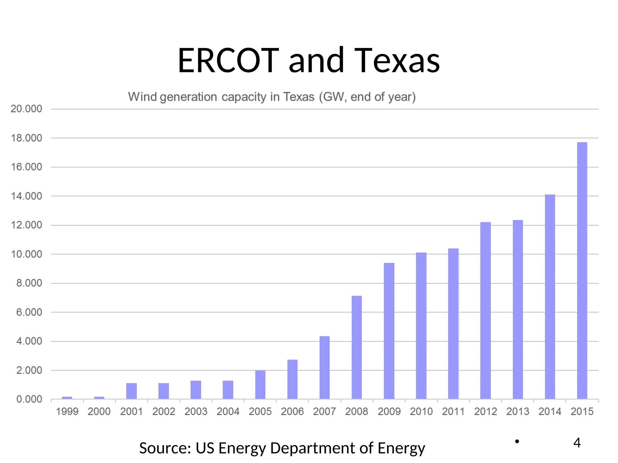
5. ERCOT
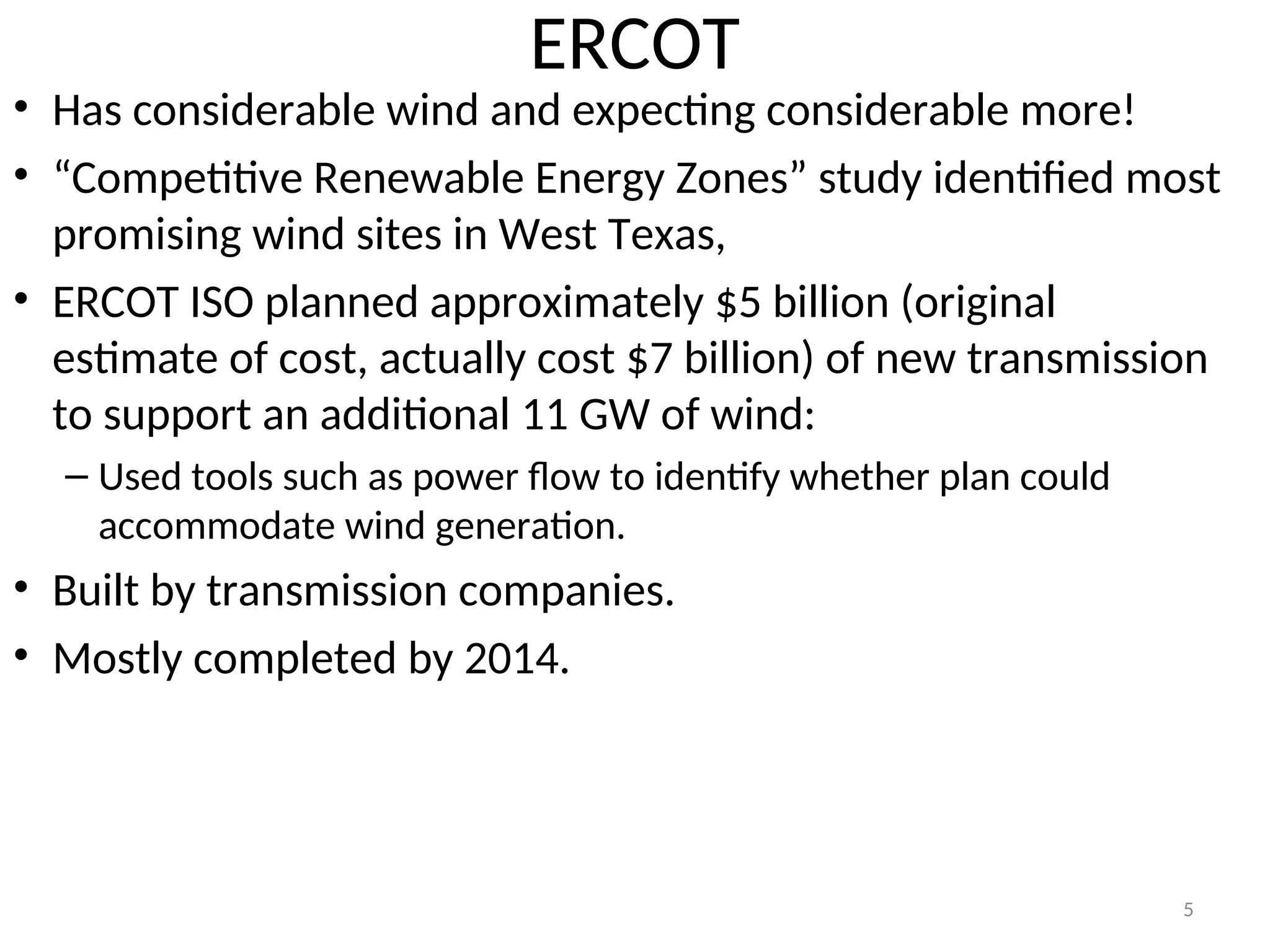
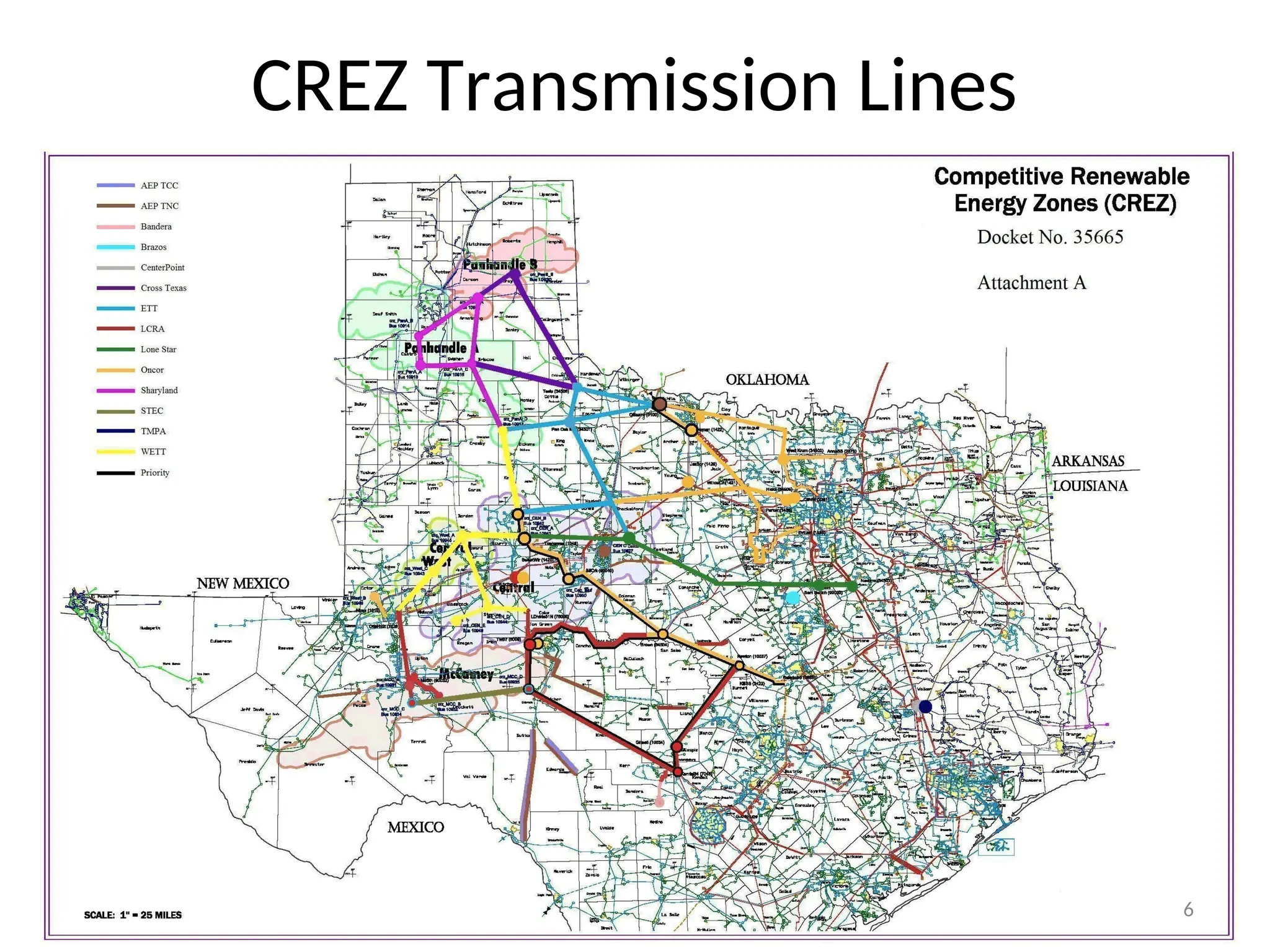
• Has considerable wind and expecting considerable more!
• “Competitive Renewable Energy Zones” study identified most
promising wind sites in West Texas,
• ERCOT ISO planned approximately $5 billion (original
estimate of cost, actually cost $7 billion) of new transmission
to support an additional 11 GW of wind:
– Used tools such as power flow to identify whether plan could
accommodate wind generation.
• Built by transmission companies.
• Mostly completed by 2014.
5

6. CREZ Transmission Lines
6

7. NR Application to Power Flow
*
* * *
1 1
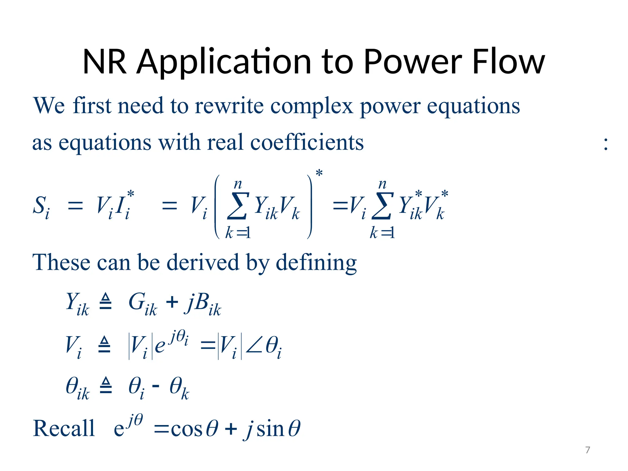
We first need to rewrite complex power equations
as equations with real coefficients (we've seen this earlier):
These can be derived by defining
n n
i i i i ik k i ik k
k k
ik ik ik
i
S V I V Y V V Y V
Y G jB
V
 
 
  
 
 

 

Recall e cos sin
i
j
i i i
ik i k
j
V e V
j



  
 
 

 


7

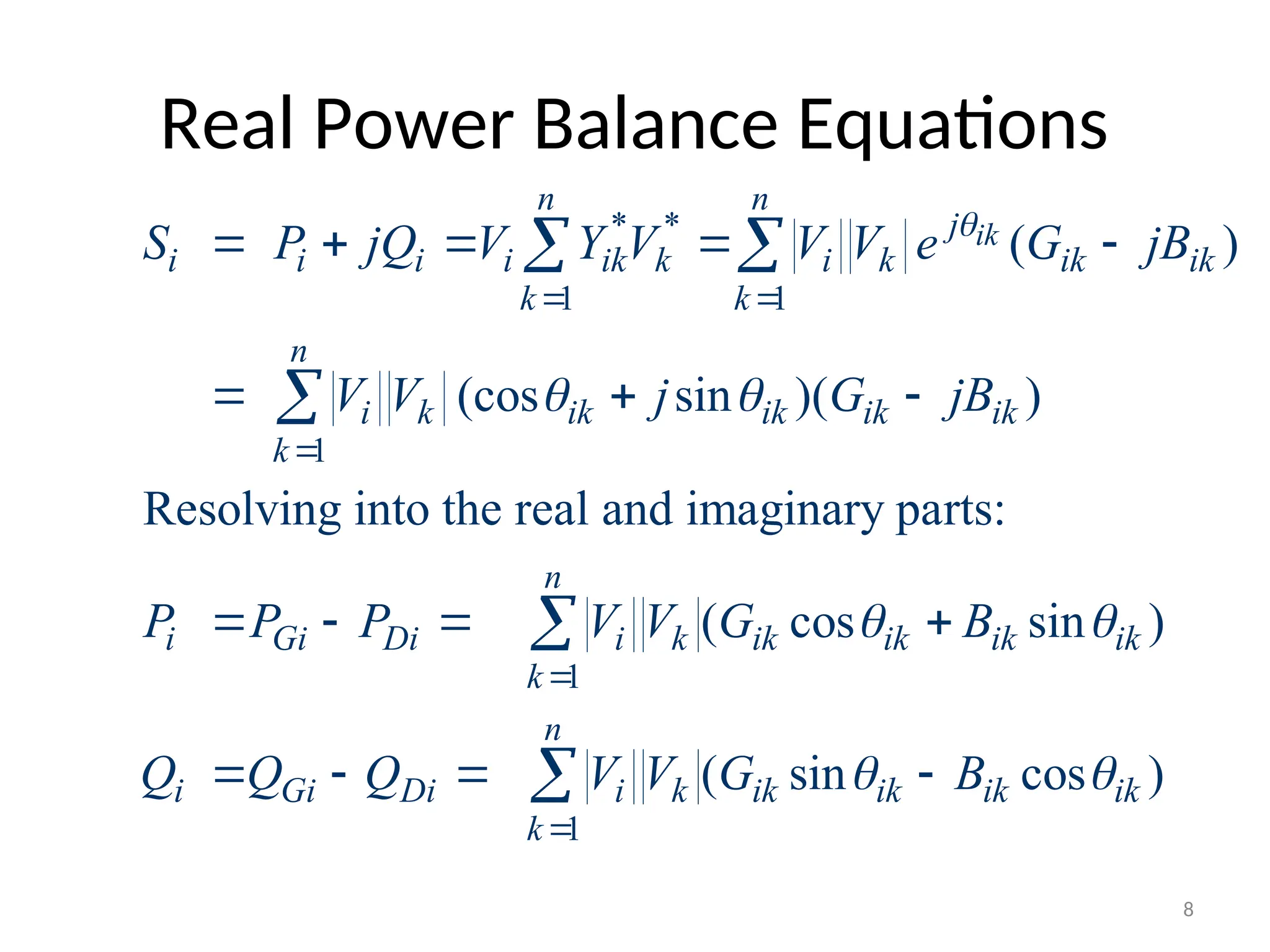
8. Real Power Balance Equations
* *
1 1
1
1
1
( )
(cos sin )( )
Resolving into the real and imaginary parts:
( cos sin )
( sin
ik
n n
j
i i i i ik k i k ik ik
k k
n
i k ik ik ik ik
k
n
i Gi Di i k ik ik ik ik
k
n
i Gi Di i k ik ik
k
S P jQ V Y V V V e G jB
V V j G jB
P P P V V G B
Q Q Q V V G

 
 

 



    
  
   
  
 


 cos )
ik ik
B 

8

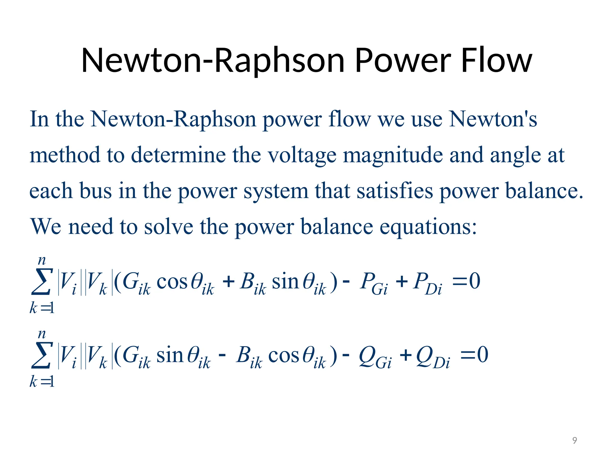
9. Newton-Raphson Power Flow
In the Newton-Raphson power flow we use Newton's
method to determine the voltage magnitude and angle at
each bus in the power system that satisfies power balance.
We need to solve the power balance equ
1
1
ations:
( cos sin ) 0
( sin cos ) 0
n
i k ik ik ik ik Gi Di
k
n
i k ik ik ik ik Gi Di
k
V V G B P P
V V G B Q Q
 
 


   
   


9

10. Power Balance Equations
• 10
1
1
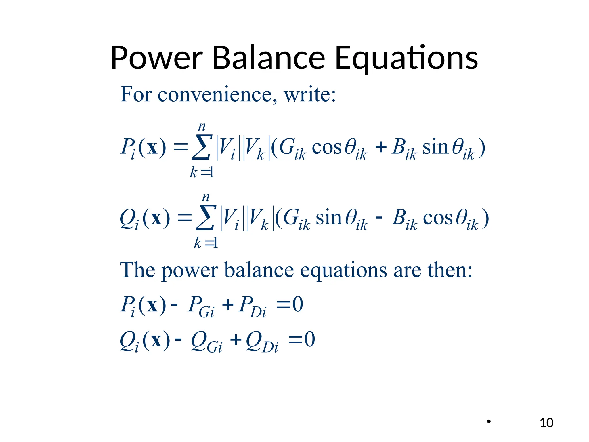
For convenience, write:
( ) ( cos sin )
( ) ( sin cos )
The power balance equations are then:
( ) 0
( ) 0
n
i i k ik ik ik ik
k
n
i i k ik ik ik ik
k
i Gi Di
i Gi Di
P V V G B
Q V V G B
P P P
Q Q Q
 
 


 
 
  
  


x
x
x
x

11. Power Balance Equations
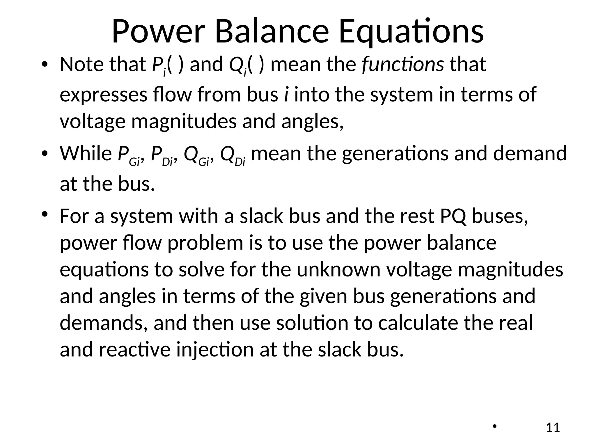
• Note that Pi( ) and Qi( ) mean the functions that
expresses flow from bus i into the system in terms of
voltage magnitudes and angles,
• While PGi, PDi, QGi, QDi mean the generations and demand
at the bus.
• For a system with a slack bus and the rest PQ buses,
power flow problem is to use the power balance
equations to solve for the unknown voltage magnitudes
and angles in terms of the given bus generations and
demands, and then use solution to calculate the real
and reactive injection at the slack bus.
• 11

12. Power Flow Variables
2
n
2
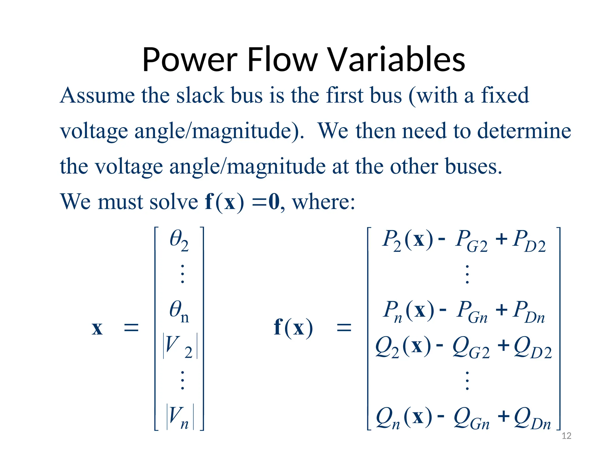
Assume the slack bus is the first bus (with a fixed
voltage angle/magnitude). We then need to determine
the voltage angle/magnitude at the other buses.
We must solve ( ) , where:
n
V
V









f x 0
x


2 2 2
2 2 2
( )
( )
( )
( )
( )
G D
n Gn Dn
G D
n Gn Dn
P P P
P P P
Q Q Q
Q Q Q
 
  
  
  
 
  

   
 
   
   
   
 
 

x
x
f x
x
x


12

13. N-R Power Flow Solution
(0)
( )
( 1) ( ) ( ) 1 ( )
The power flow is solved using the same procedure
discussed previously for general equations:
For 0; make an initial guess of ,
While ( ) Do
[ ( )] ( )
1
End
v
v v v v
v
v v

 


 
 
x x
f x
x x J x f x
13

14. Power Flow Jacobian Matrix
1 1 1
1 2 2 2
2 2 2
1 2 2 2
2 2 2 2 2 2
1 2
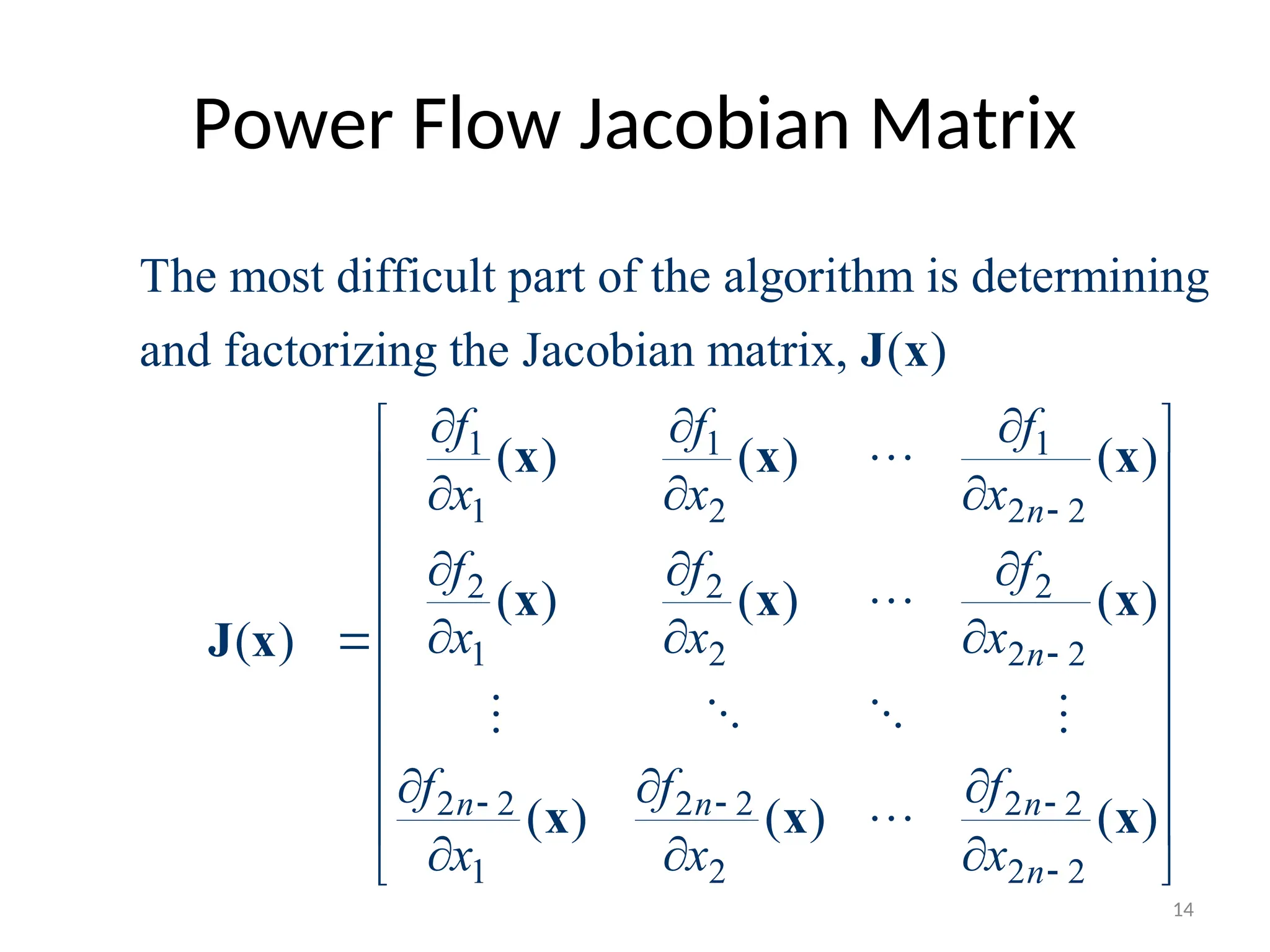
The most difficult part of the algorithm is determining
and factorizing the Jacobian matrix, ( )
( ) ( ) ( )
( ) ( ) ( )
( )
( ) ( )
n
n
n n n
f f f
x x x
f f f
x x x
f f f
x x x


  
  
  
  
  

  
  
J x
x x x
x x x
J x
x x


   

2 2
( )
n
 
 
 
 
 
 
 
 
 
 
x
14

15. Power Flow Jacobian Matrix,
cont’d
1
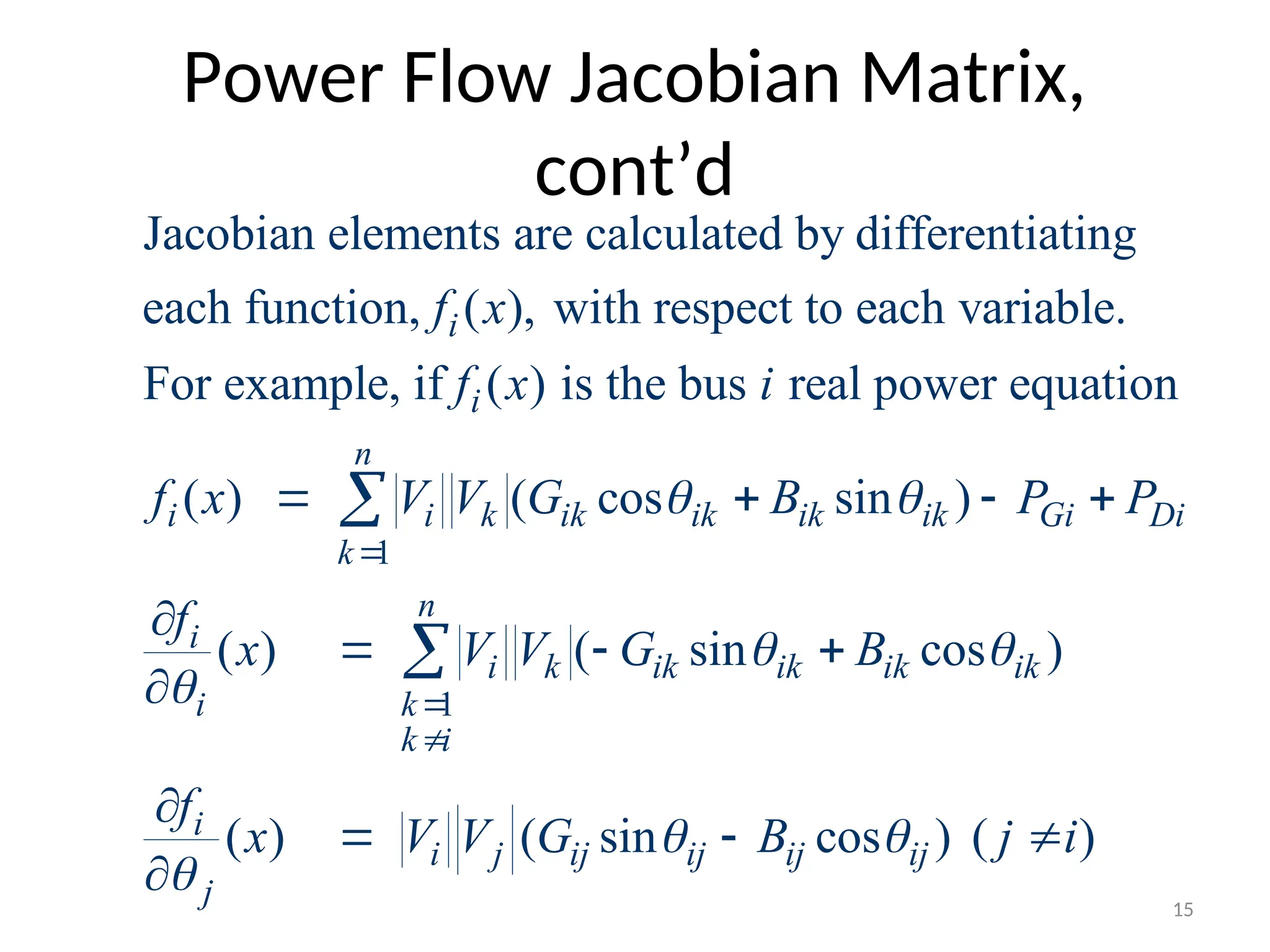
Jacobian elements are calculated by differentiating
each function, ( ), with respect to each variable.
For example, if ( ) is the bus real power equation
( ) ( cos sin )
i
i
n
i i k ik ik ik ik Gi
k
f x
f x i
f x V V G B P P
 

   

1
( ) ( sin cos )
( ) ( sin cos ) ( )
Di
n
i
i k ik ik ik ik
i k
k i
i
i j ij ij ij ij
j
f
x V V G B
f
x V V G B j i
 

 




  


  


15

16. Two Bus Newton-Raphson
Example
Line Z = 0.1j
One Two
1.000 pu 1.000 pu
200 MW
100 MVR
0 MW
0 MVR
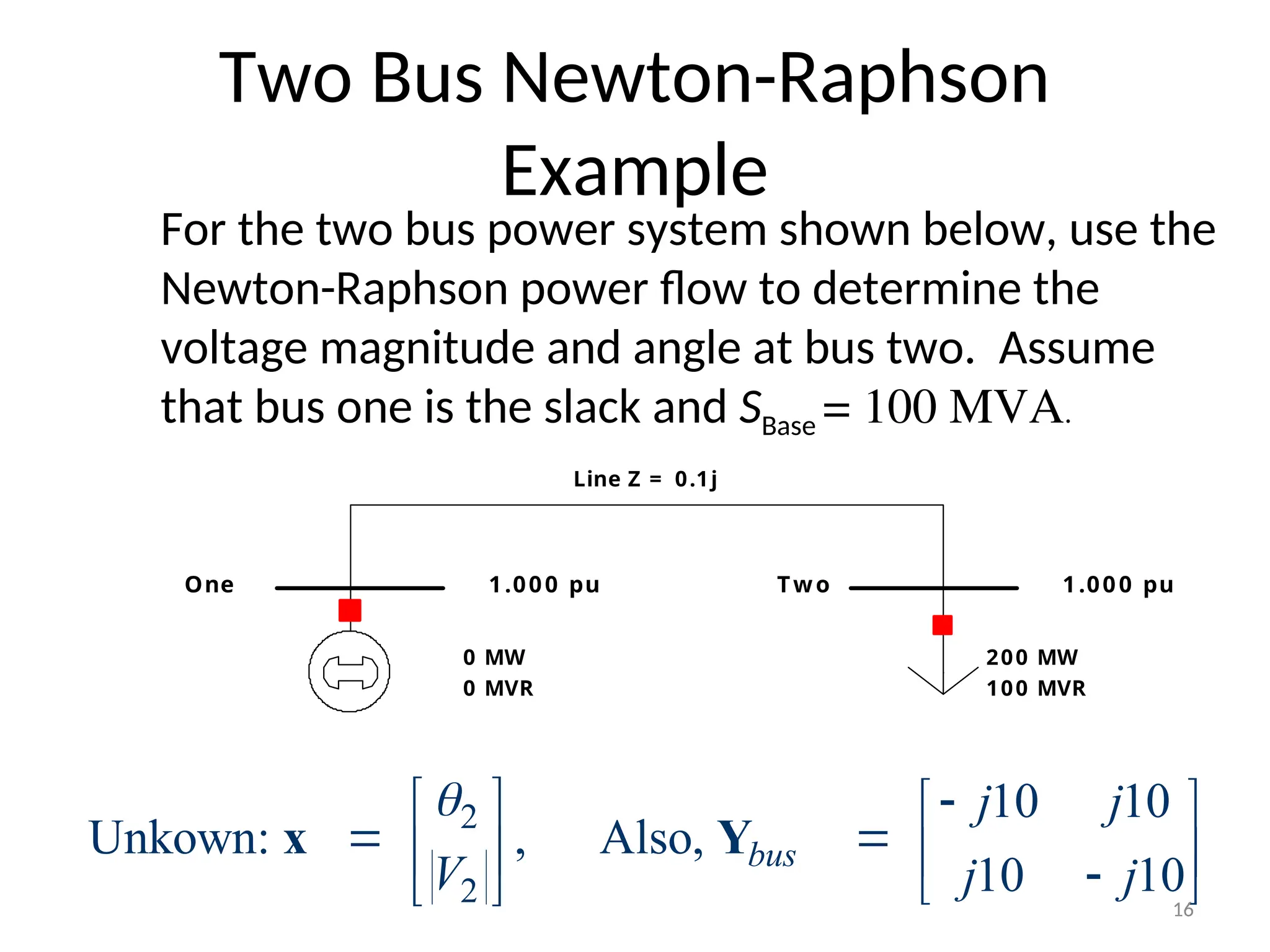
For the two bus power system shown below, use the
Newton-Raphson power flow to determine the
voltage magnitude and angle at bus two. Assume
that bus one is the slack and SBase = 100 MVA.
2
2
10 10
Unkown: , Also,
10 10
bus
j j
V j j
 
   
 
   

 
 
x Y
16

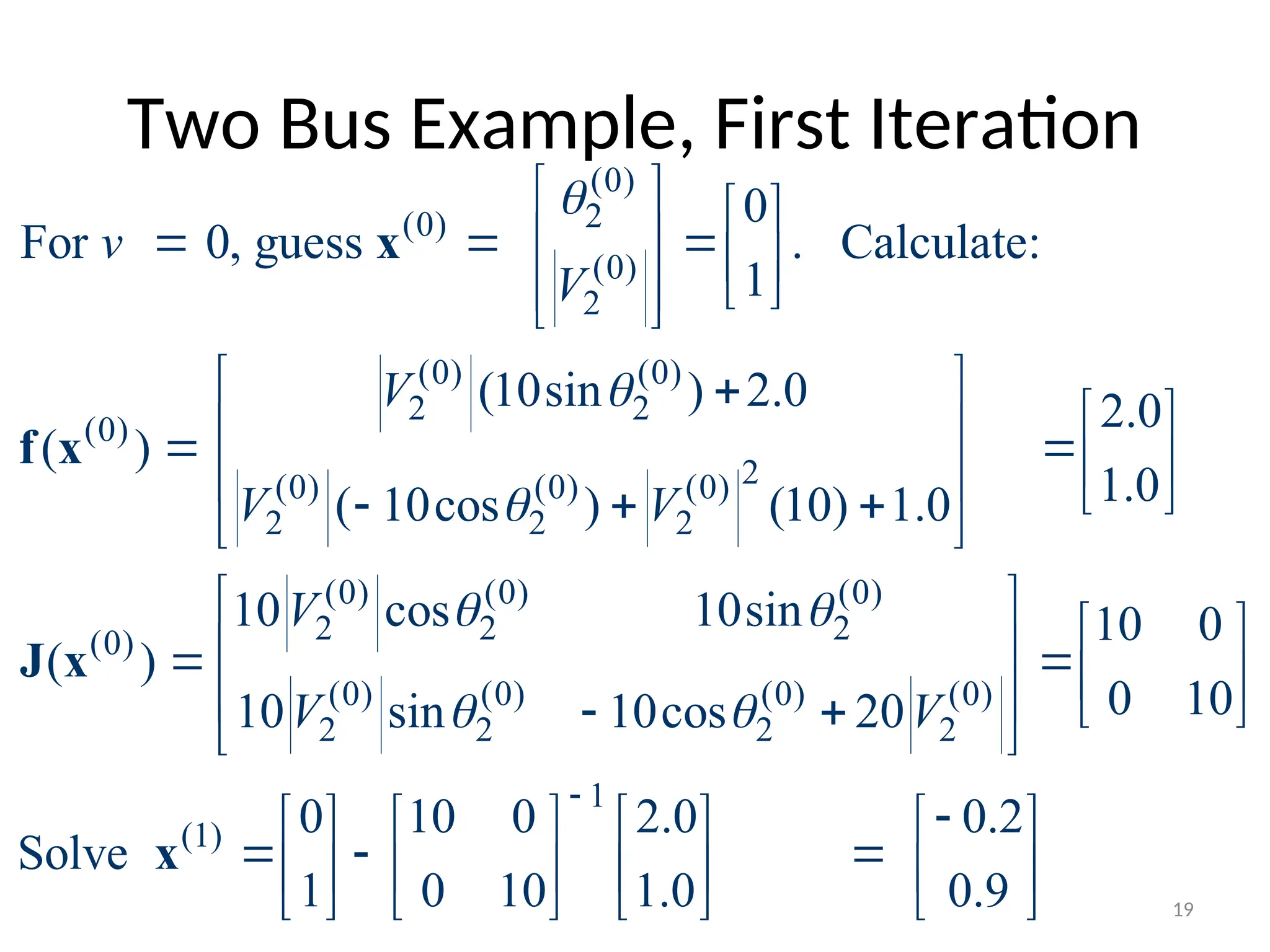
17. Two Bus Example, cont’d
1
1
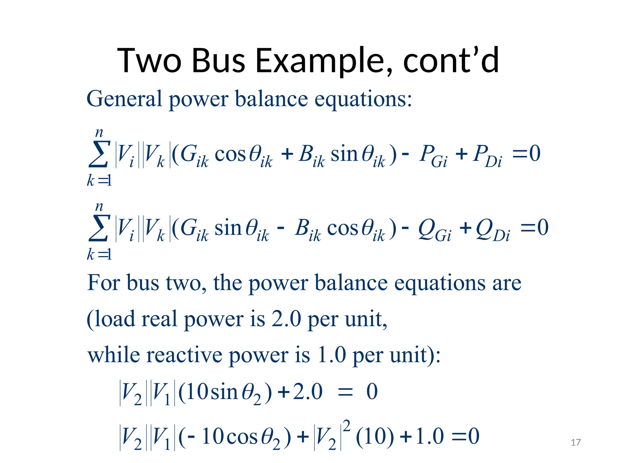
General power balance equations:
( cos sin ) 0
( sin cos ) 0
For bus two, the power balance equations are
(load real power is 2.0 per unit,
while react
n
i k ik ik ik ik Gi Di
k
n
i k ik ik ik ik Gi Di
k
V V G B P P
V V G B Q Q
 
 


   
   


2 1 2
2
2 1 2 2
ive power is 1.0 per unit):
(10sin ) 2.0 0
( 10cos ) (10) 1.0 0
V V
V V V


 
    17

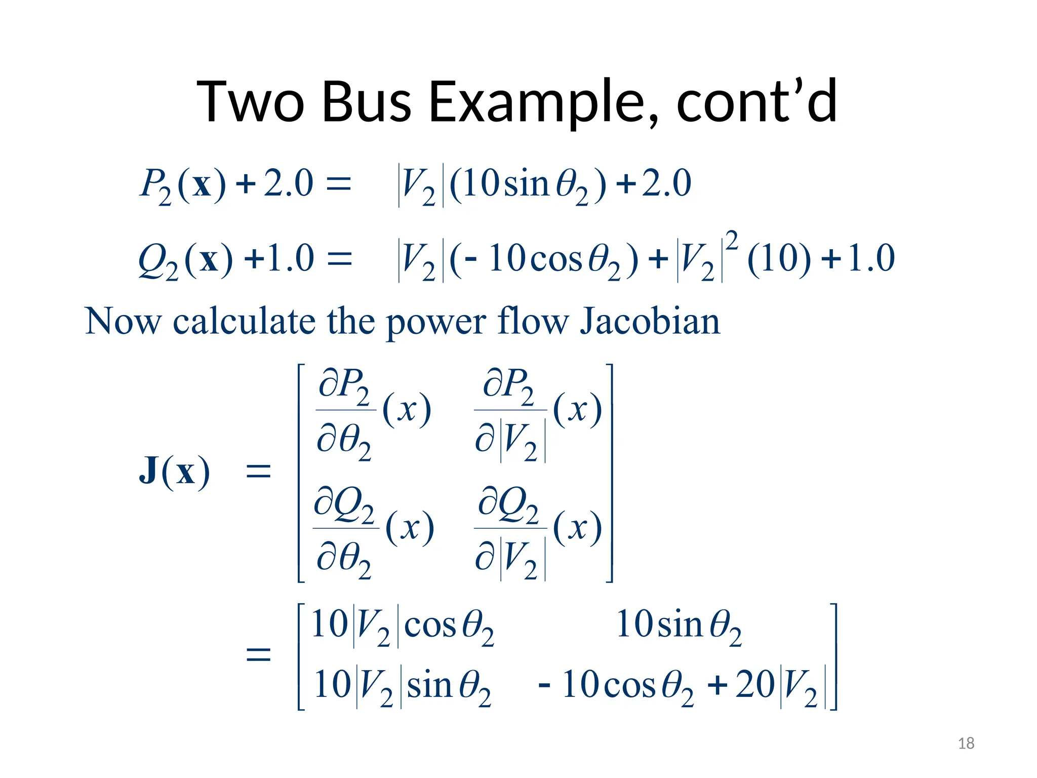
18. Two Bus Example, cont’d
2 2 2
2
2 2 2 2
2 2
2 2
2 2
2 2
2 2 2
2 2 2 2
( ) 2.0 (10sin ) 2.0
( ) 1.0 ( 10cos ) (10) 1.0
Now calculate the power flow Jacobian
( ) ( )
( )
( ) ( )
10 cos 10sin
10 sin 10cos 20
P V
Q V V
P P
x x
V
Q Q
x x
V
V
V V




 
 
  
    
 
 
 
 
 

 
 
 
 
 
 
  
 
 
x
x
J x
18

19. Two Bus Example, First Iteration
(0)
2
(0)
(0)
2
(0) (0)
2 2
(0)
2
(0) (0) (0)
2 2 2
(0) (0) (0)
2 2 2
(0)
(0) (0)
2 2
0
For 0, guess . Calculate:
1
(10sin ) 2.0 2.0
( )
1.0
( 10cos ) (10) 1.0
10 cos 10sin
( )
10 sin 10cos
v
V
V
V V
V
V



 

   
  
   
 
 
 
 

 
 
  
   
  
 


x
f x
J x
(0) (0)
2 2
1
(1)
10 0
0 10
20
0 10 0 2.0 0.2
Solve
1 0 10 1.0 0.9
V


 
 
   
   

 

       
  
       
       
x
19

20. Two Bus Example, Next Iterations
(1)
2
(1)
1
(2)
0.9(10sin( 0.2)) 2.0 0.212
( )
0.279
0.9( 10cos( 0.2)) 0.9 10 1.0
8.82 1.986
( )
1.788 8.199
0.2 8.82 1.986 0.212 0.233
0.9 1.788 8.199 0.279 0.8586
(

 
   
 
   
      
 

 
  

 
  
       
  
       

       
f x
J x
x
f (2) (3)
(3)
2
0.0145 0.236
)
0.0190 0.8554
0.0000906
( ) Close enough! 0.8554 13.52
0.0001175
V

   
 
   
   
 
    
 
 
x x
f x
20

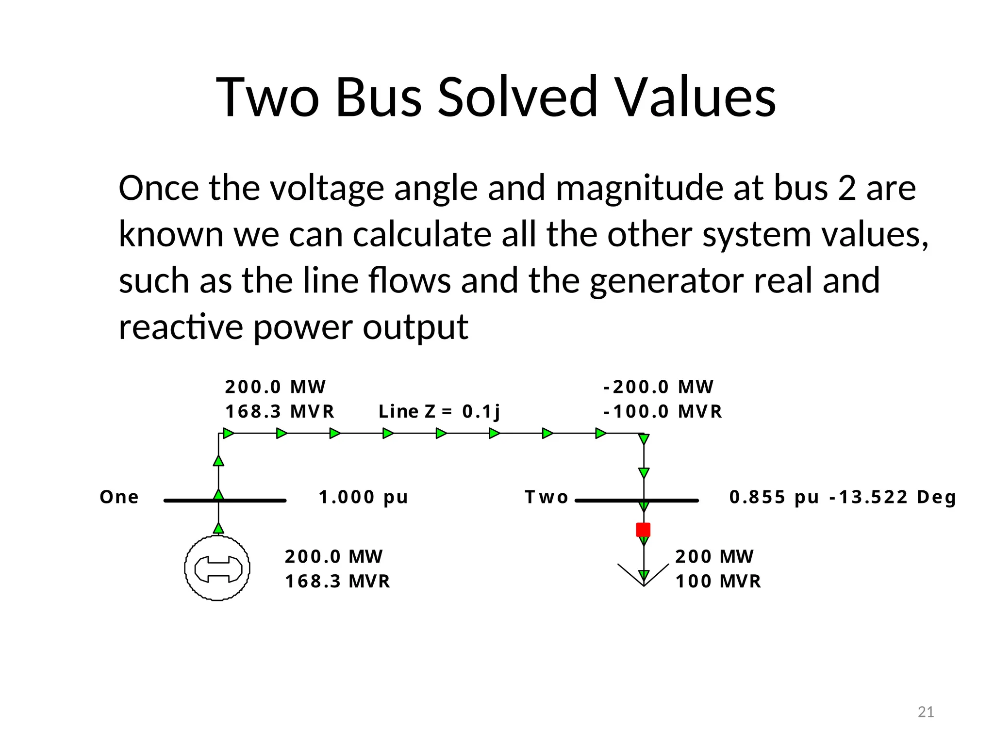
21. Two Bus Solved Values
Line Z = 0.1j
One T wo
1.000 pu 0.855 pu
200 MW
100 MVR
200.0 MW
168.3 MVR
- 13.522 Deg
200.0 MW
168.3 MVR
- 200.0 MW
- 100.0 MVR
Once the voltage angle and magnitude at bus 2 are
known we can calculate all the other system values,
such as the line flows and the generator real and
reactive power output
21

22. Two Bus Case Low Voltage Solution
(0)
(0) (0)
2 2
(0)
(0) (0) (0
2 2 2
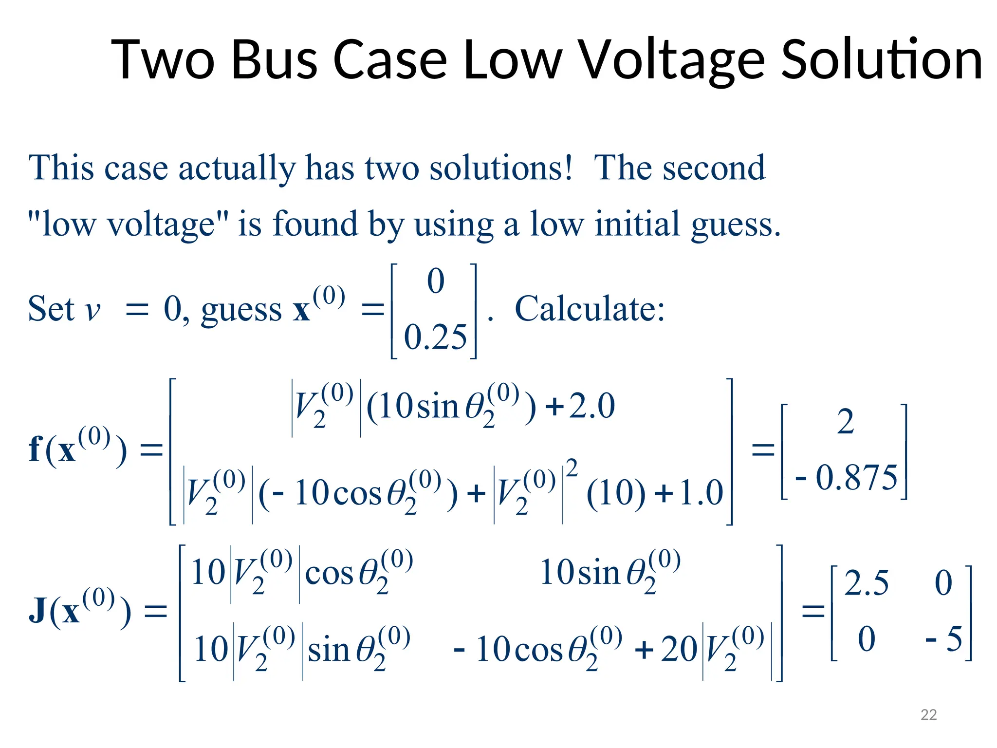
This case actually has two solutions! The second
"low voltage" is found by using a low initial guess.
0
Set 0, guess . Calculate:
0.25
(10sin ) 2.0
( )
( 10cos )
v
V
V V


 
  
 


 
x
f x 2
)
(0) (0) (0)
2 2 2
(0)
(0) (0) (0) (0)
2 2 2 2
2
0.875
(10) 1.0
10 cos 10sin 2.5 0
( )
0 5
10 sin 10cos 20
V
V V
 
 
 
 
   
  
 

 
 
 
 
  

   
 
 
J x
22

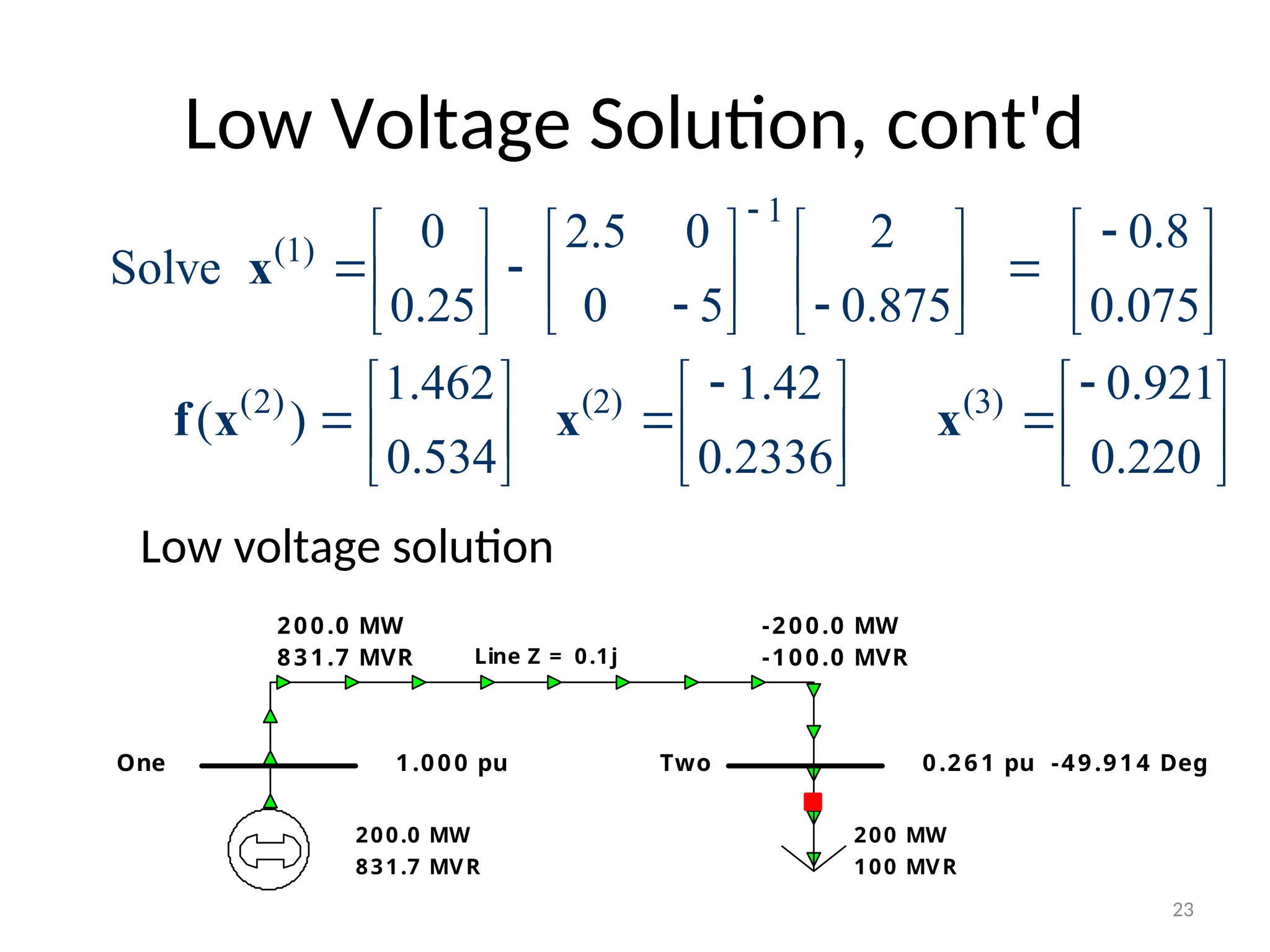
23. Low Voltage Solution, cont'd
1
(1)
(2) (2) (3)
0 2.5 0 2 0.8
Solve
0.25 0 5 0.875 0.075
1.462 1.42 0.921
( )
0.534 0.2336 0.220


       
  
       
 
       
 
     
  
     
     
x
f x x x
Line Z = 0.1j
One Two
1.000 pu 0.261 pu
200 MW
100 MVR
200.0 MW
831.7 MVR
-49.914 Deg
200.0 MW
831.7 MVR
-200.0 MW
-100.0 MVR
Low voltage solution
23

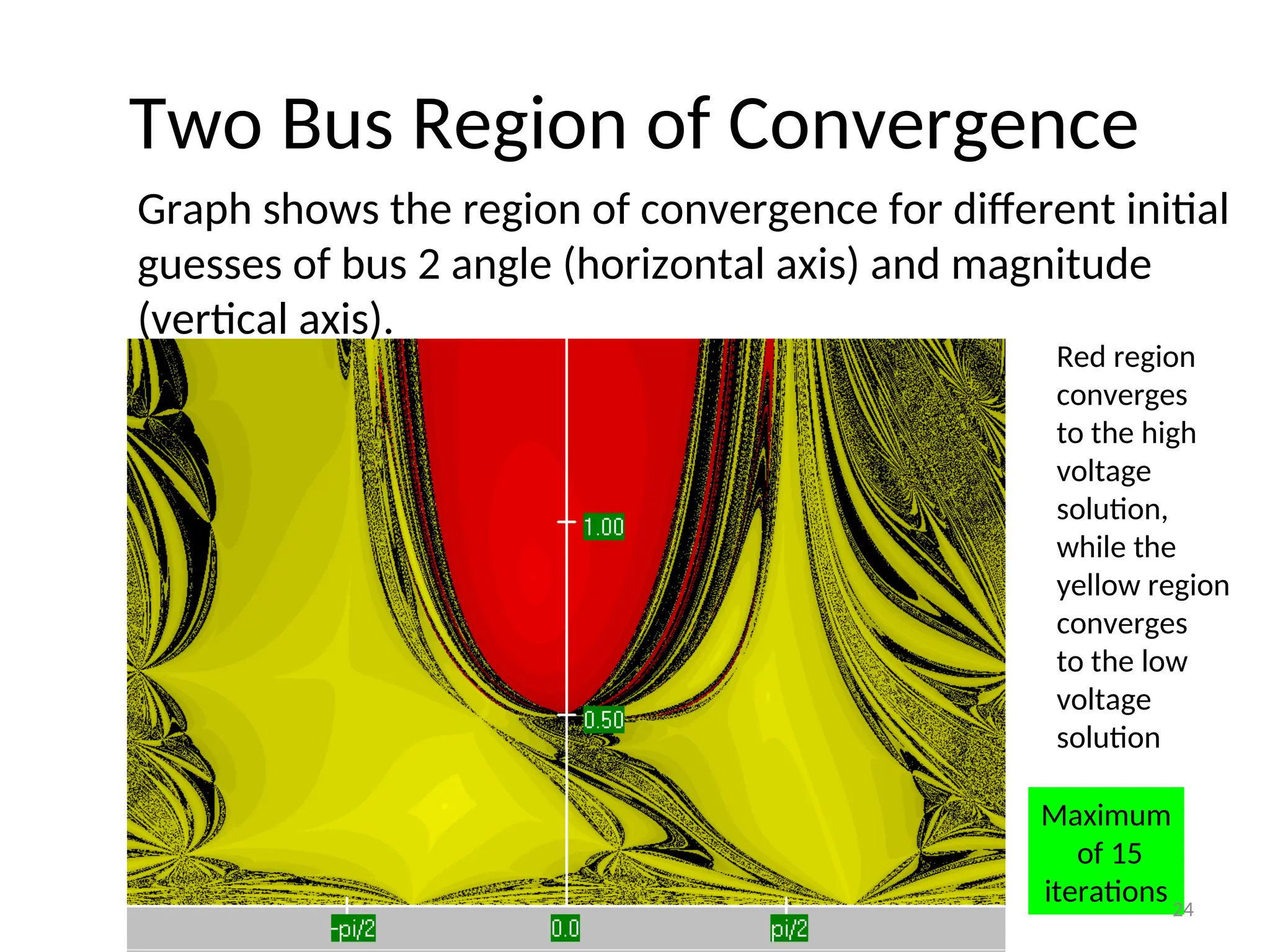
24. Two Bus Region of Convergence
Graph shows the region of convergence for different initial
guesses of bus 2 angle (horizontal axis) and magnitude
(vertical axis).
Red region
converges
to the high
voltage
solution,
while the
yellow region
converges
to the low
voltage
solution
Maximum
of 15
iterations24

25. PV Buses
Since the voltage magnitude at PV buses is fixed there is no need
to explicitly include these voltages in x nor explicitly include the
reactive power balance equations at the PV buses:
– the reactive power output of the generator varies to maintain the fixed
terminal voltage (within limits), so we can just use the solved voltages
and angles to calculate the reactive power production to be whatever is
needed to satisfy reactive power balance.
– An alternative is to keep the reactive power balance equation explicit
but also write an explicit voltage constraint for the generator bus:
|Vi | – Vi setpoint = 0
25

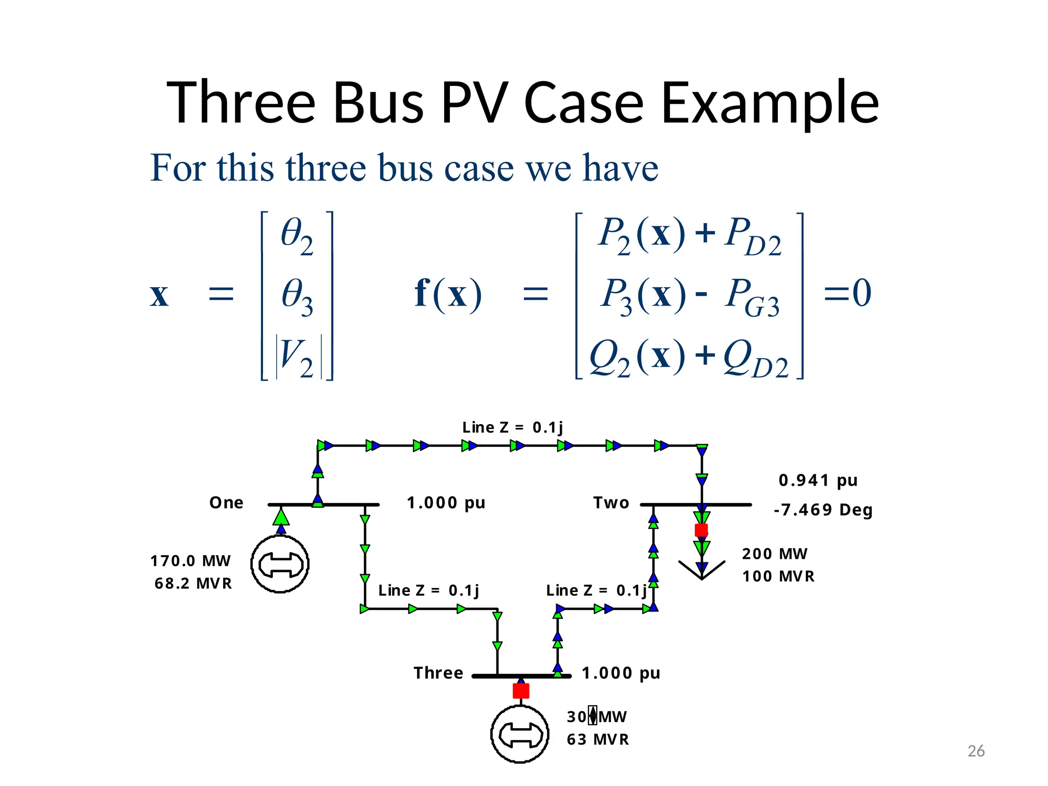
26. Three Bus PV Case Example
Line Z = 0.1j
Line Z = 0.1j Line Z = 0.1j
One Two
1.000 pu
0.941 pu
200 MW
100 MVR
170.0 MW
68.2 MVR
-7.469 Deg
Three 1.000 pu
30 MW
63 MVR
2 2 2
3 3 3
2 2 2
For this three bus case we have
( )
( ) ( ) 0
( )
D
G
D
P P
P P
V Q Q



   
   
   
   

 
   
 
x
x f x x
x
26

27. PV Buses
• With Newton-Raphson, PV buses means that there are
less unknown variables we need to calculate explicitly
and less equations we need to satisfy explicitly.
• Reactive power balance is satisfied implicitly by
choosing reactive power production to be whatever is
needed, once we have a solved case (like real and
reactive power at the slack bus).
• Contrast to Gauss iterations where PV buses
complicated the algorithm.
27

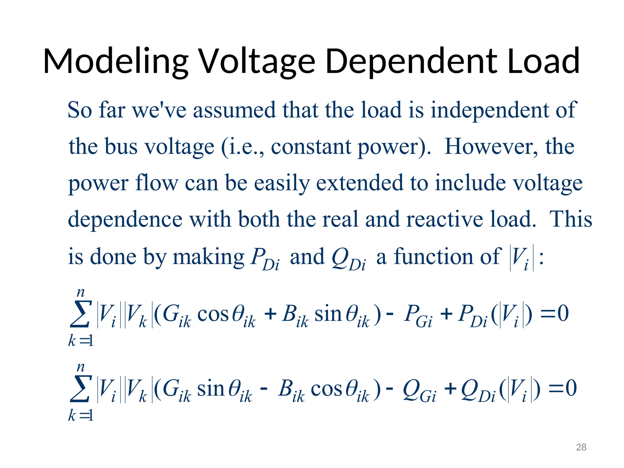
28. Modeling Voltage Dependent Load
So far we've assumed that the load is independent of
the bus voltage (i.e., constant power). However, the
power flow can be easily extended to include voltage
dependence with both the real and reactive
1
1
load. This
is done by making and a function of :
( cos sin ) ( ) 0
( sin cos ) ( ) 0
Di Di i
n
i k ik ik ik ik Gi Di i
k
n
i k ik ik ik ik Gi Di i
k
P Q V
V V G B P P V
V V G B Q Q V
 
 


   
   


28

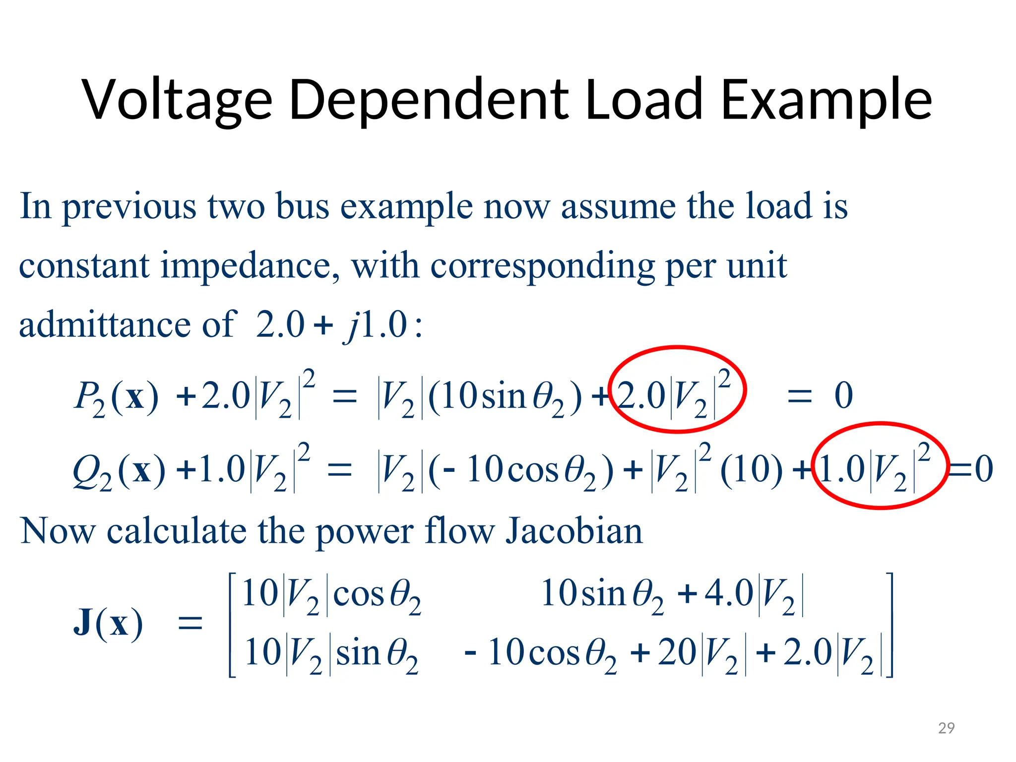
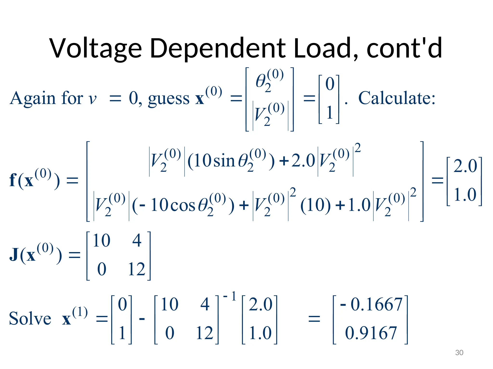
29. Voltage Dependent Load Example
2 2
2 2 2 2 2
2 2 2
2 2 2 2 2 2
In previous two bus example now assume the load is
constant impedance, with corresponding per unit
admittance of 2.0 1.0:
( ) 2.0 (10sin ) 2.0 0
( ) 1.0 ( 10cos ) (10) 1.0 0
Now
j
P V V V
Q V V V V



   
     
x
x
2 2 2 2
2 2 2 2 2
calculate the power flow Jacobian
10 cos 10sin 4.0
( )
10 sin 10cos 20 2.0
V V
V V V
 
 

 
  
  
 
J x
29

30. Voltage Dependent Load, cont'd
(0)
2
(0)
(0)
2
2
(0) (0) (0)
2 2 2
(0)
2 2
(0) (0) (0) (0)
2 2 2 2
(0)
(1)
0
Again for 0, guess . Calculate:
1
(10sin ) 2.0 2.0
( )
1.0
( 10cos ) (10) 1.0
10 4
( )
0 12
0
Solve
1
v
V
V V
V V V



   
  
   
 
 
 
 
  
 
  
   
  
 
 
 
 
 



x
f x
J x
x
1
10 4 2.0 0.1667
0 12 1.0 0.9167


      
 
      
      
30

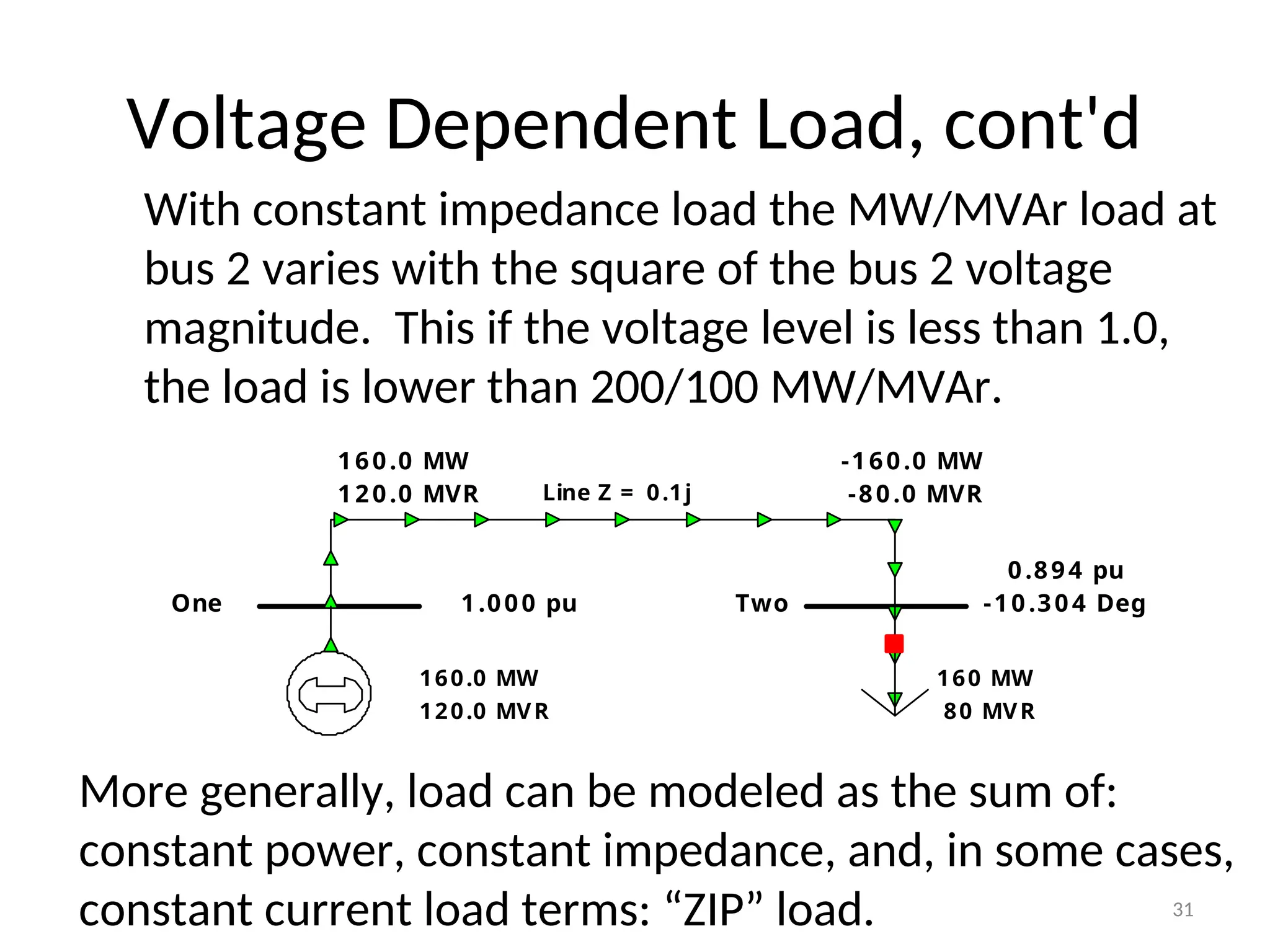
31. Voltage Dependent Load, cont'd
Line Z = 0.1j
One Two
1.000 pu
0.894 pu
160 MW
80 MVR
160.0 MW
120.0 MVR
-10.304 Deg
160.0 MW
120.0 MVR
-160.0 MW
-80.0 MVR
With constant impedance load the MW/MVAr load at
bus 2 varies with the square of the bus 2 voltage
magnitude. This if the voltage level is less than 1.0,
the load is lower than 200/100 MW/MVAr.
31
More generally, load can be modeled as the sum of:
constant power, constant impedance, and, in some cases,
constant current load terms: “ZIP” load.

32. Solving Large Power Systems
Most difficult computational task is inverting the
Jacobian matrix (or solving the update equation):
– factorizing a full matrix is an order n3
operation, meaning the
amount of computation increases with the cube of the size of
the problem.
– this amount of computation can be decreased substantially by
recognizing that since Ybus is a sparse matrix, the Jacobian is
also a sparse matrix.
– using sparse matrix methods results in a computational order
of about n1.5
.
– this is a substantial savings when solving systems with tens of
thousands of buses.
32

33. Newton-Raphson Power Flow
Advantages
– fast convergence as long as initial guess is close to
solution
– large region of convergence
Disadvantages
– each iteration takes much longer than a Gauss-Seidel
iteration
– more complicated to code, particularly when
implementing sparse matrix algorithms
Newton-Raphson algorithm is very common in
power flow analysis.
33