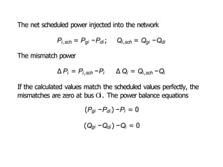
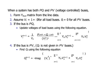
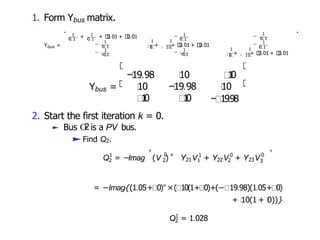
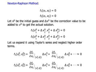
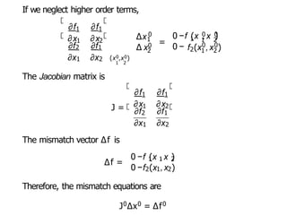
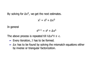
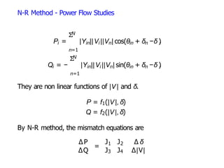
Power flow studies analyze the steady state operation of power systems by calculating the voltage magnitude and angle at each bus. They use numerical methods like Gauss-Seidel and Newton-Raphson to solve the nonlinear power flow equations iteratively. Power flow studies classify buses as load buses with specified real and reactive power, generator/voltage controlled buses that control voltage magnitude, and a reference slack bus that balances the system.

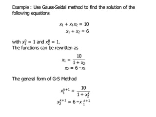
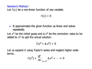
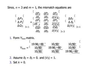
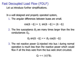
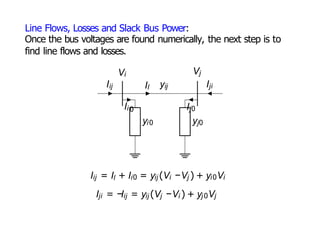
![where
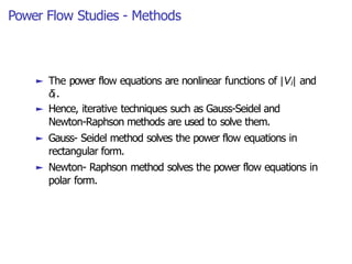
∆P = Psch −Pcal; ∆Q = Qsch −Qcal
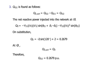
J1, J2, J3 and J4 are sub matrices of Jacobian.
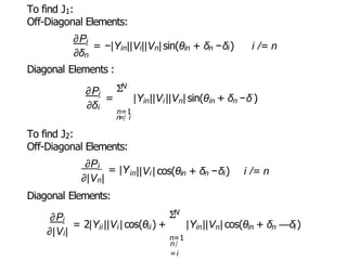
∂P ∂P ∂Q ∂Q
J1 = [
∂δ
]; J2 = [
∂|V |
]; J3 = [
∂δ
]; J4 = [
∂|V |
];
(n −1) × 1.
To find the size of the Jacobian matrix, let us assume that there
are m voltage controlled buses in the system of n buses.
► Since P is specified for n −1 buses, the size of ∆P is
► Since Q is specified for only PQ buses, the size of ∆Q is
(n −m −1) × 1.
► Size of J1 is (n −1) × (n −1)
► Size of J2 is (n −1) × (n −m −1)
► Size of J3 is (n −m −1) × (n −1)
► Size of J4 is (n −m −1) × (n −m −1)
The size of the Jacobian is (2n −m −2) × (2n −m −2).](https://image.slidesharecdn.com/loadflow-230425055109-c06e4e91/85/Load_Flow-pptx-35-320.jpg)


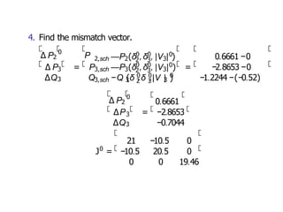
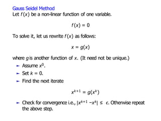
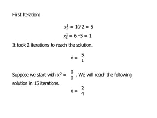
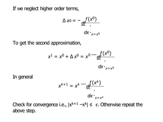
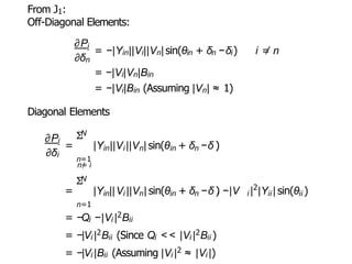
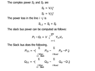
![5. Solve for the correction vector.
∆ δ2
0
3
∆|V3|
0 −1
∆ δ = [J ] ∆ P
∆ P2
0
3
∆Q3
∆ δ2
0
3
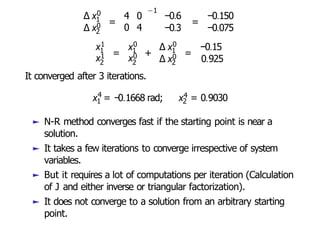
∆ δ = −0.1660 rad
−0.0513 rad
∆|V3| −0.0362
6. Find the new estimate.
δ2
1
3
δ = δ + ∆ δ
δ2
0
3 3
|V3| |V3| ∆|V3|
∆ δ2
0
δ2
1
3
|V3| 1 −0.0362
δ = 0 + −0.1660 = −0.1660 rad
0.9638
0 −0.0513 −0.0513 rad](https://image.slidesharecdn.com/loadflow-230425055109-c06e4e91/85/Load_Flow-pptx-42-320.jpg)
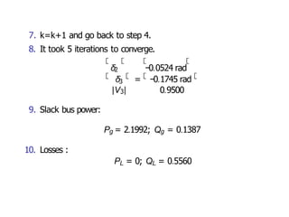
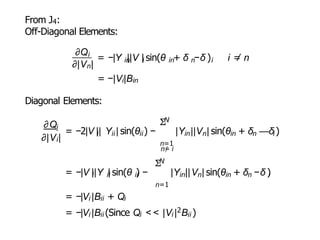
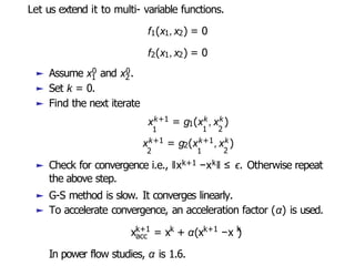
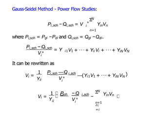
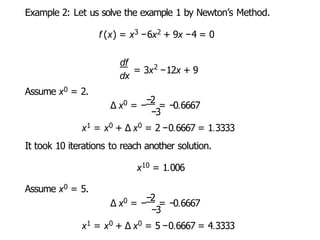
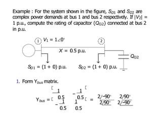
![Therefore,
|V|
∆P
= −BJ∆ δ
∆Q
= −BJJ∆ |V|
|V|
1. BJ and BJJ are the imaginary part of the bus admittance
matrix (YBus ).
2. The size of BJ is (n −1) × (n −1) and the size of BJJ is
(n −m −1) × (n −m −1).
3. Since they are constant, they need to be triangulaized
(inverted) once.
∆P
∆ δ = −[BJ]−1
|V|
∆Q
∆ |V| = −[BJJ]−1
|V |](https://image.slidesharecdn.com/loadflow-230425055109-c06e4e91/85/Load_Flow-pptx-48-320.jpg)


![[Deck] What's New in Spark-Iceberg Integration via DSV2.pptx](https://cdn.slidesharecdn.com/ss_thumbnails/deckwhatsnewinspark-icebergintegrationviadsv2-260210005337-25955b12-thumbnail.jpg?width=640&height=640&fit=bounds)


