Downloaded 456 times

This chapter discusses confidence interval estimation. It covers constructing confidence intervals for a single population mean when the population standard deviation is known or unknown, as well as confidence intervals for a single population proportion. The chapter defines key concepts like point estimates, confidence levels, and degrees of freedom. It provides examples of how to calculate confidence intervals using the normal, t, and binomial distributions and how to interpret the resulting intervals.
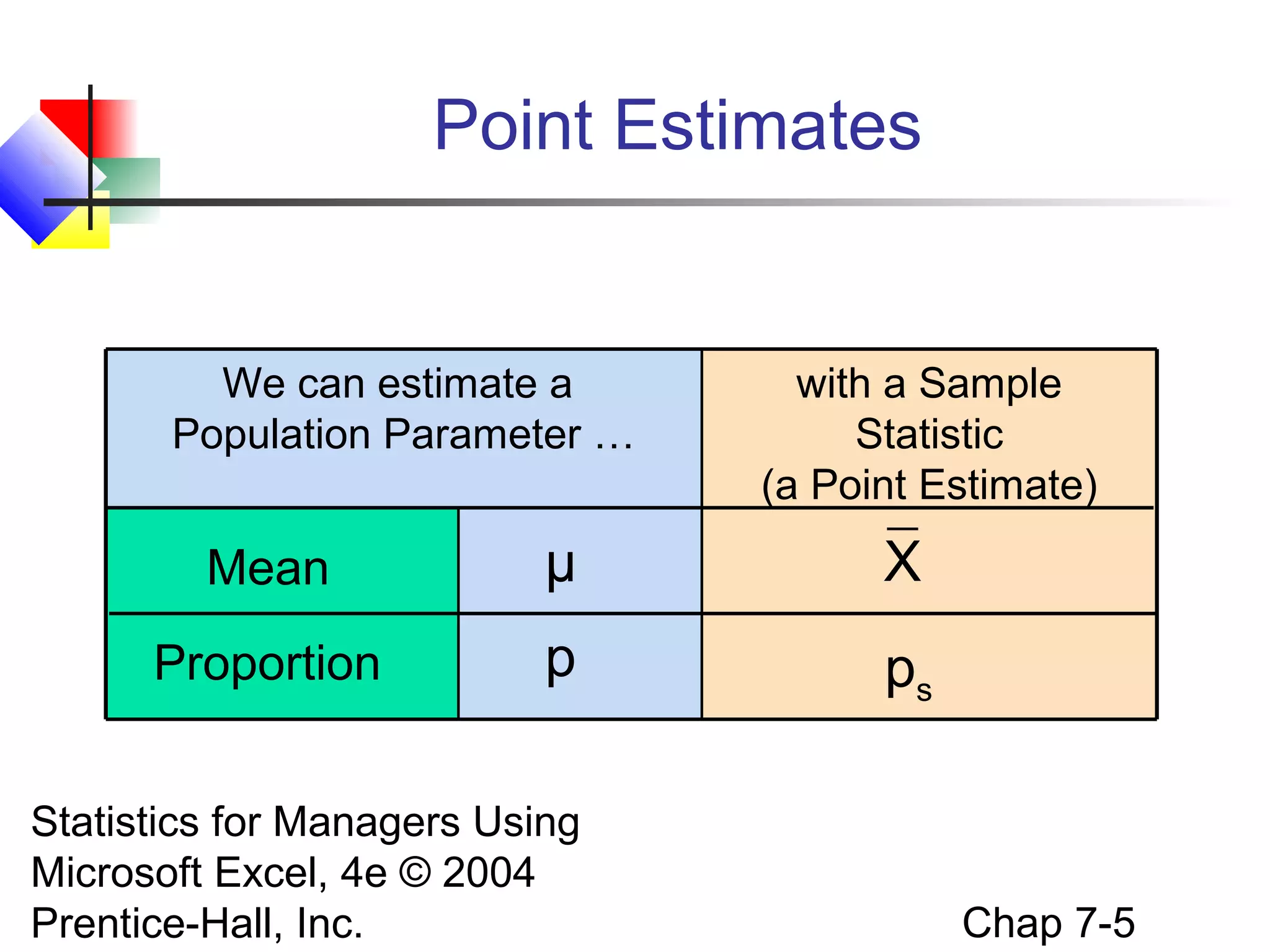
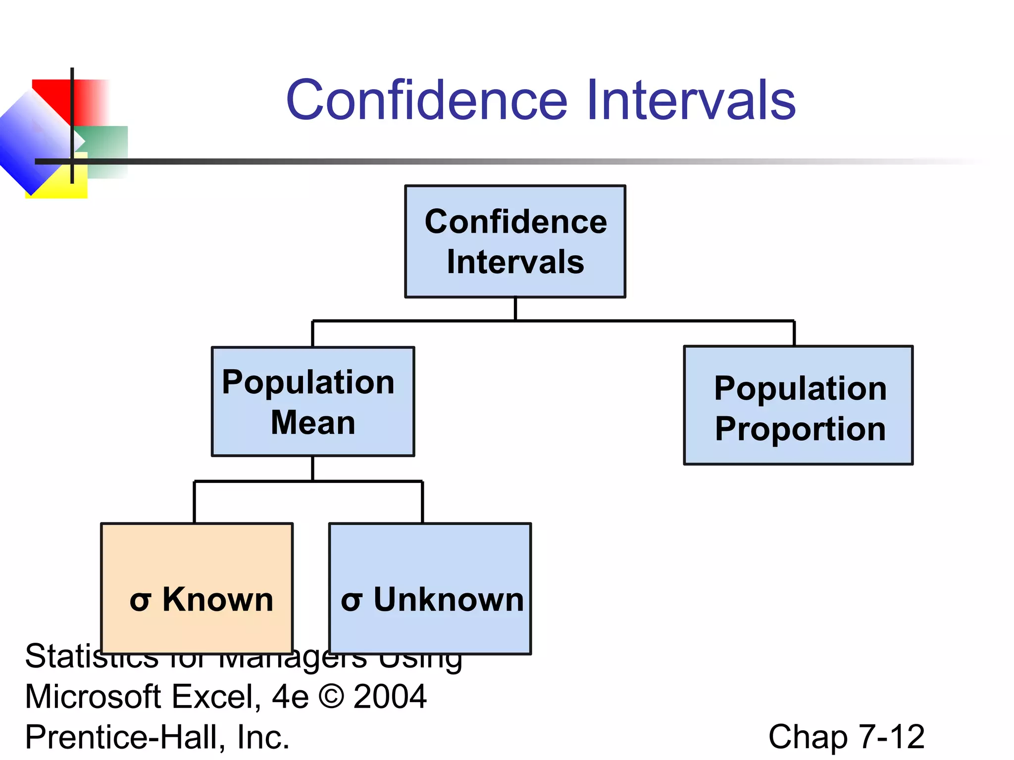
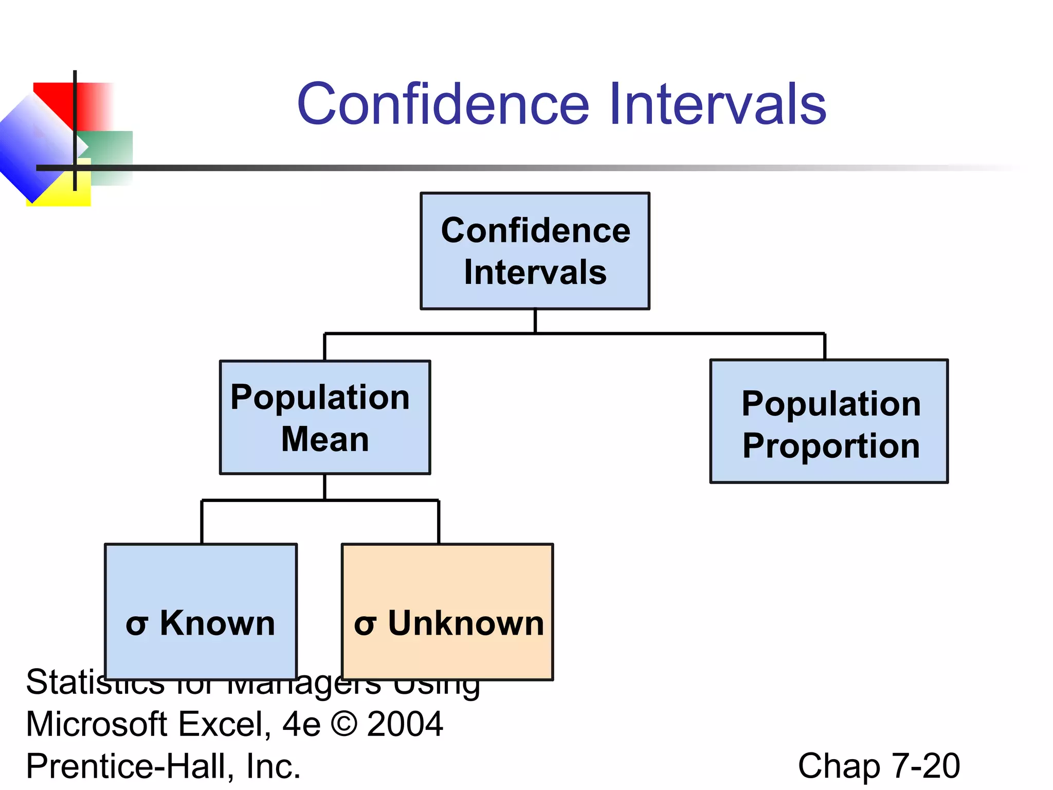
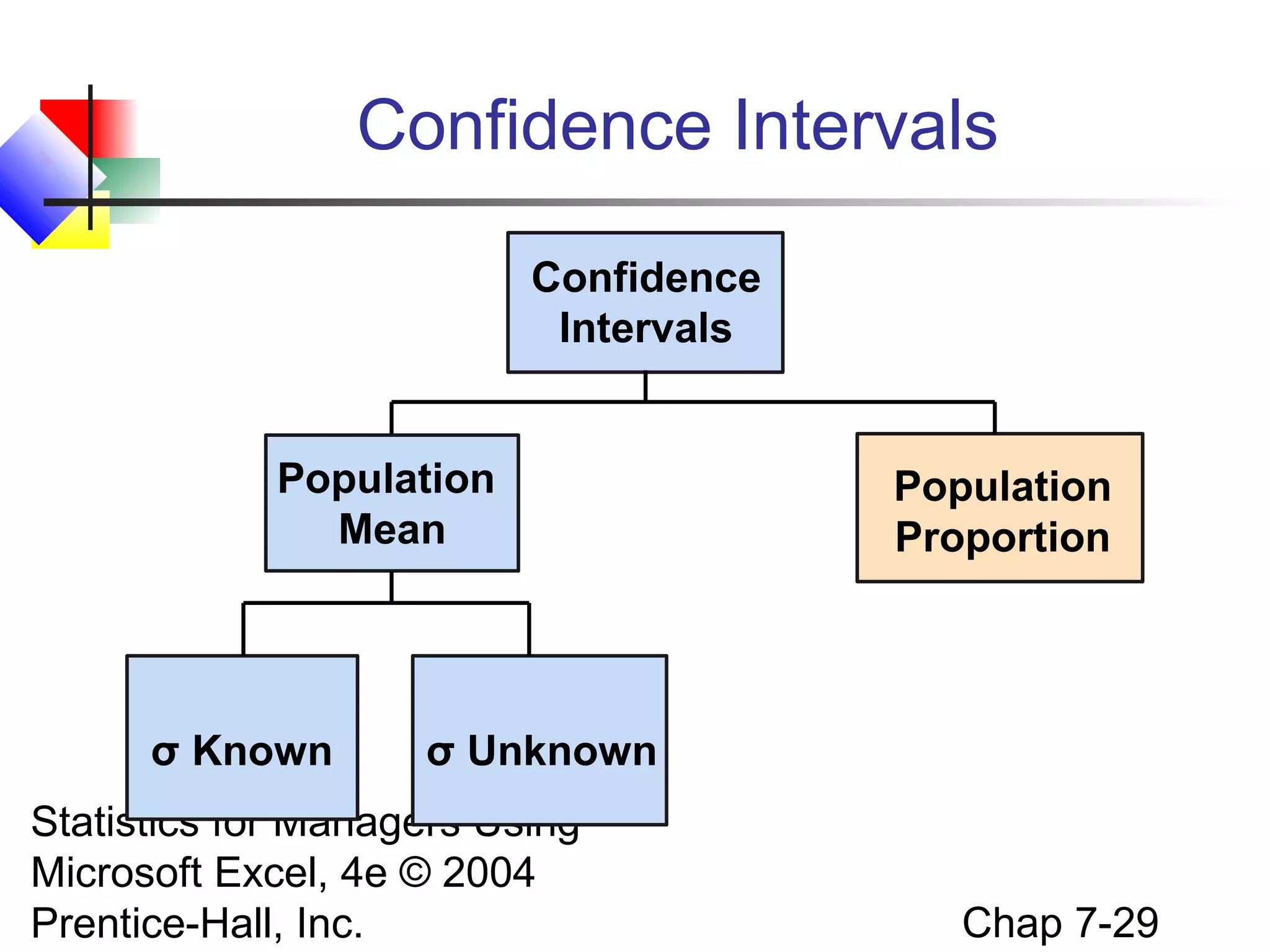
Overview of confidence intervals, types, and chapter goals.
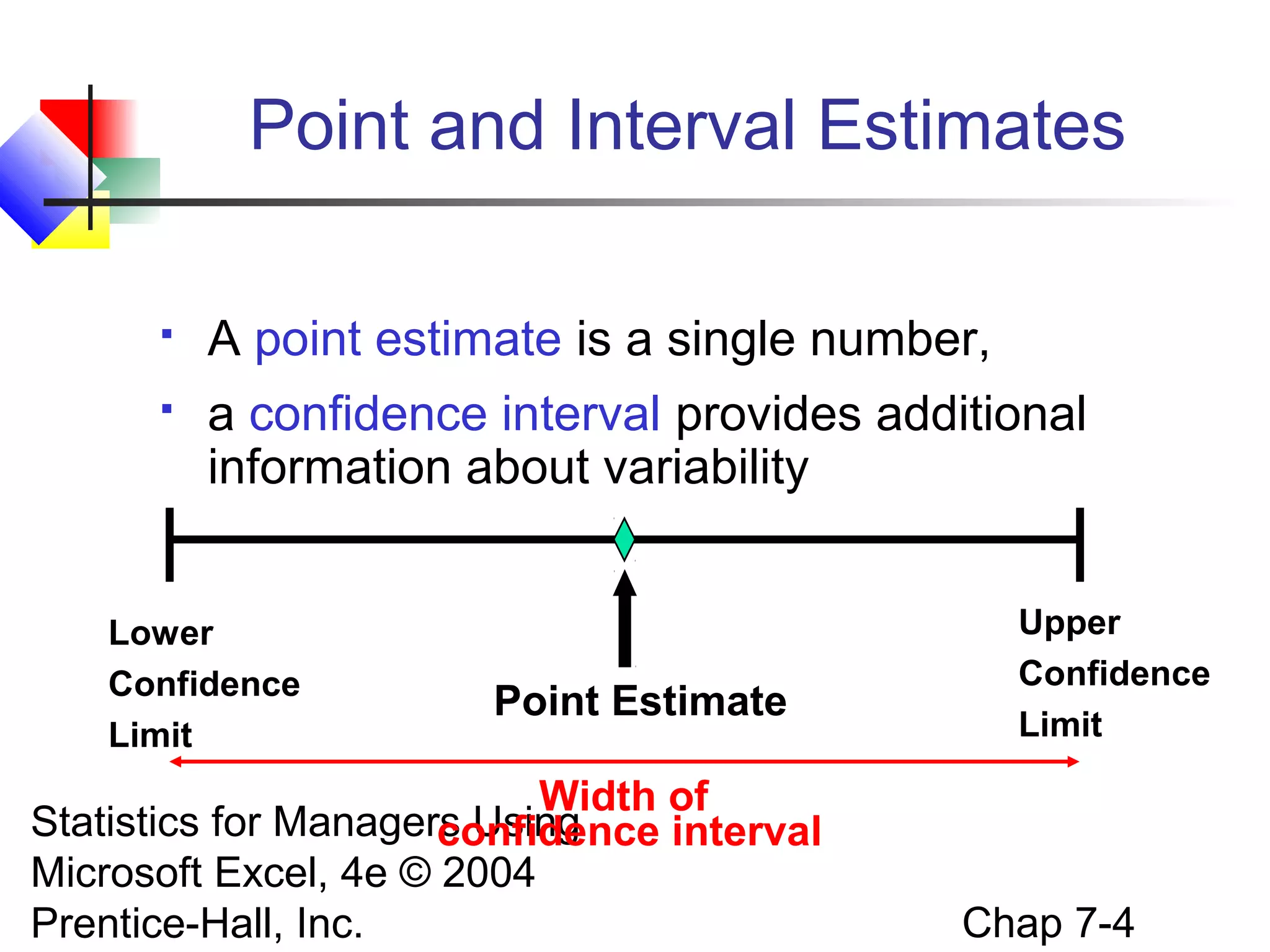
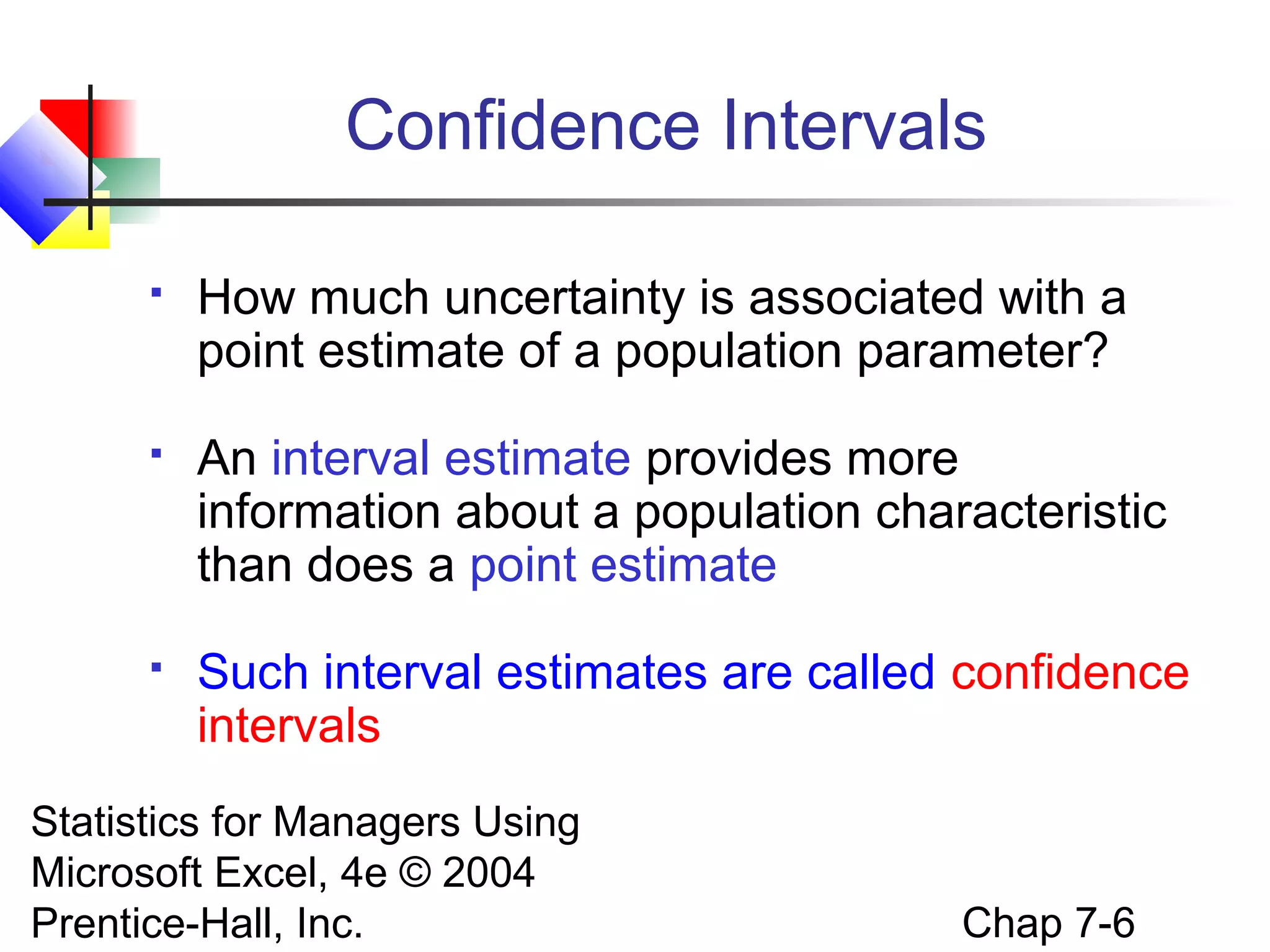
Distinction between point and interval estimates; interval estimates provide variability information.
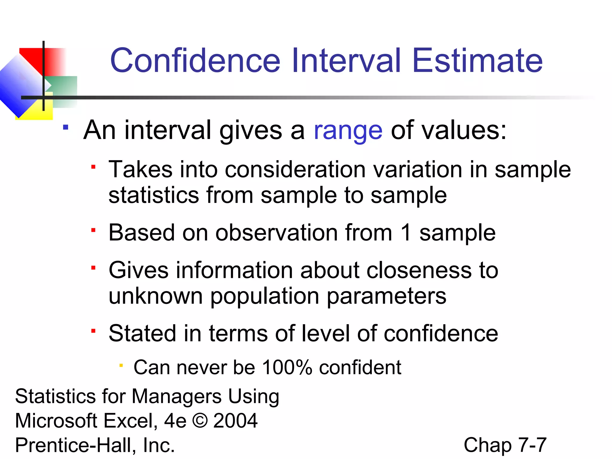
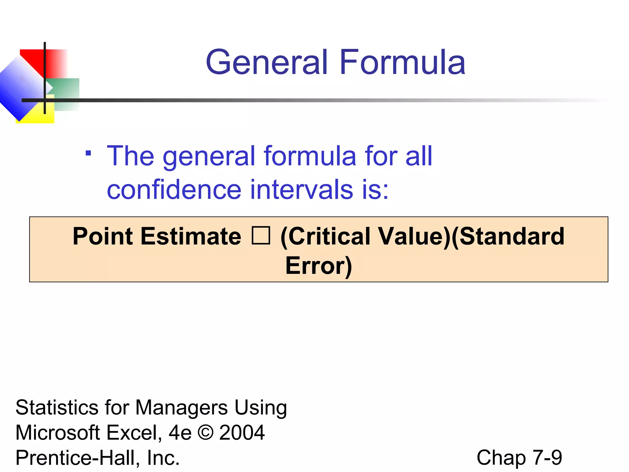
Interval estimates information, process for calculating confidence intervals, and confidence levels.
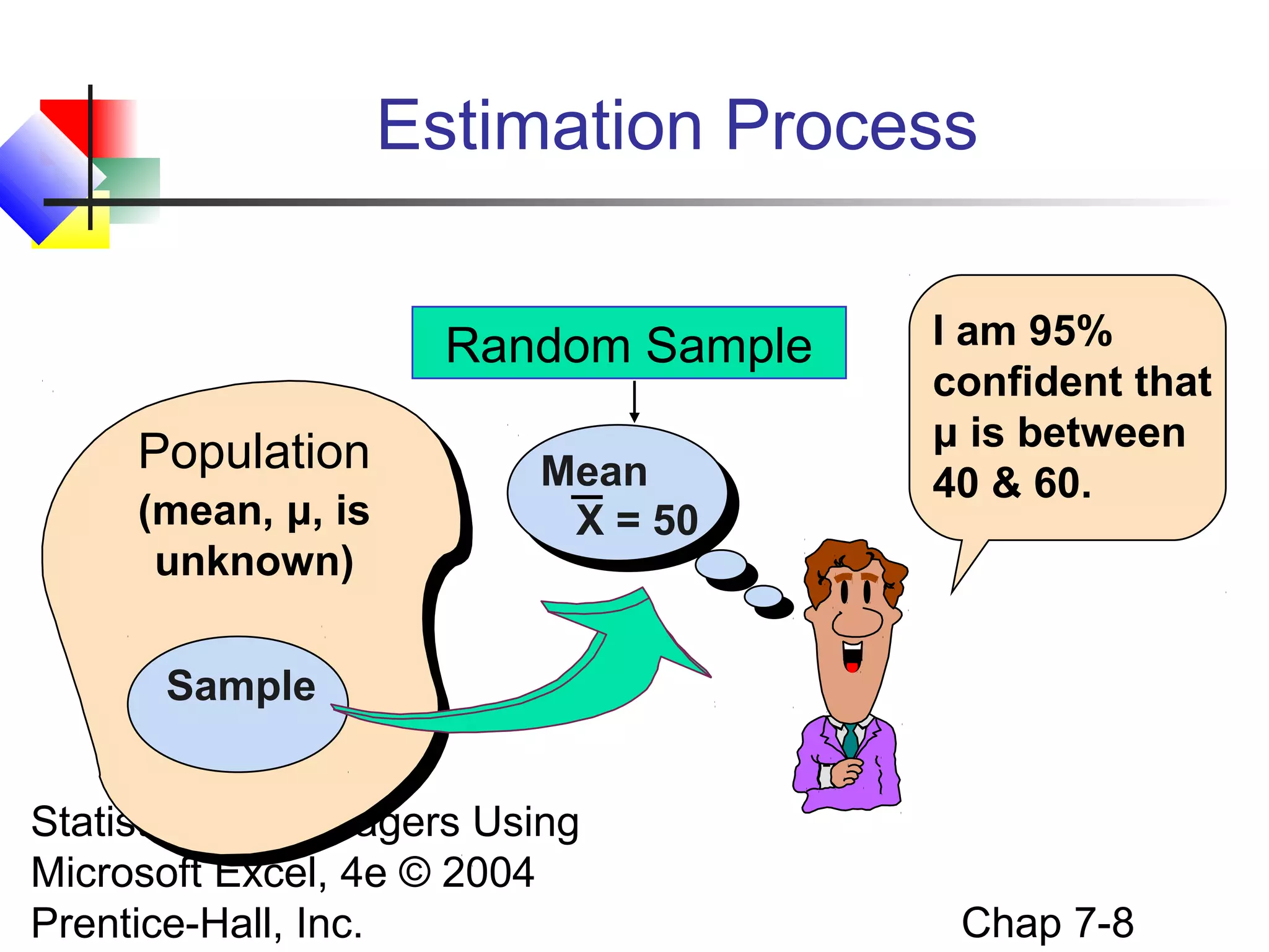
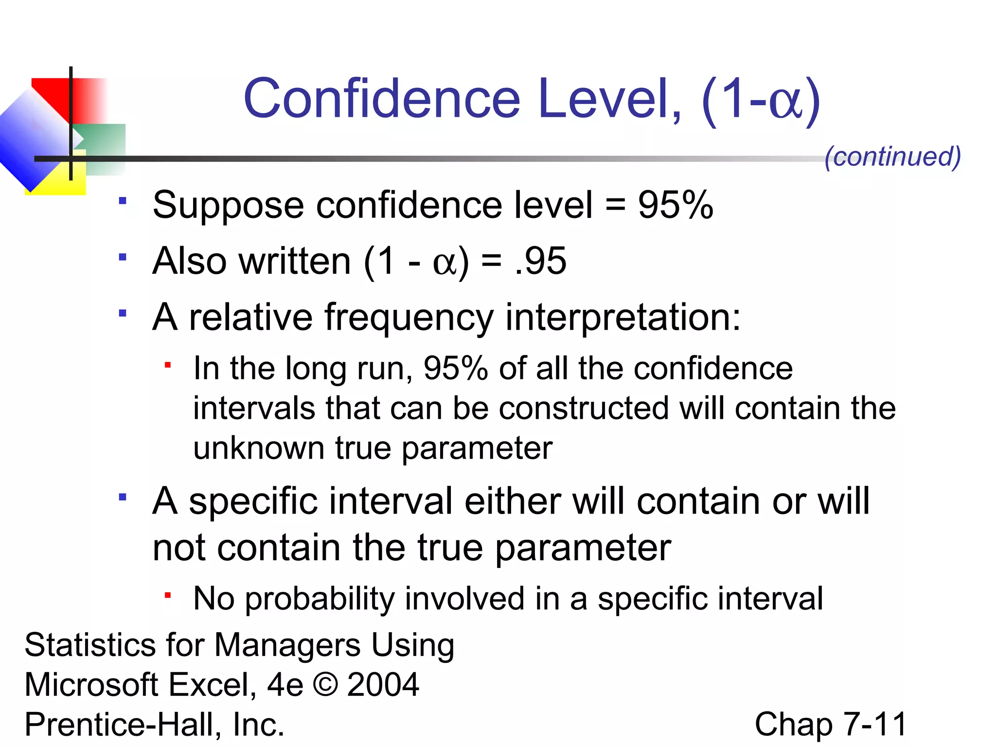
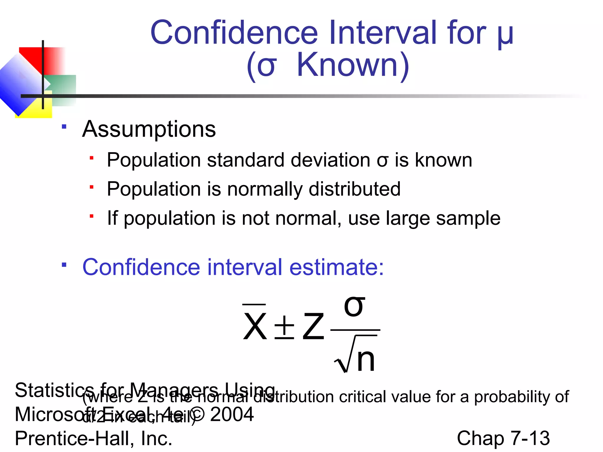
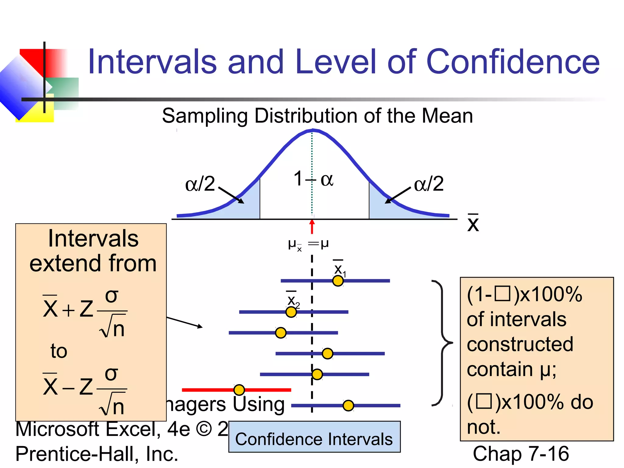
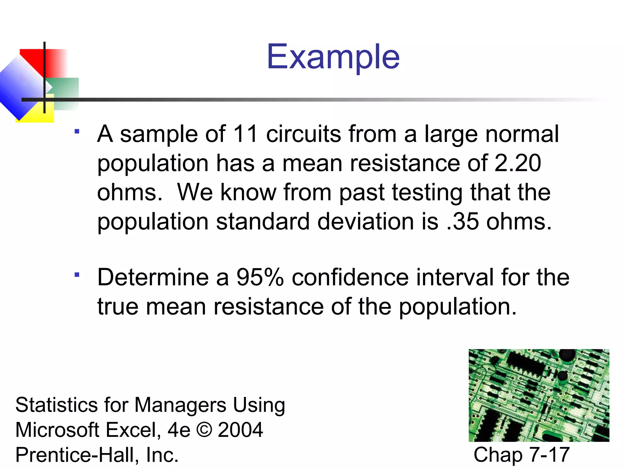
Confidence level interpretation; calculating intervals when population standard deviation is known.
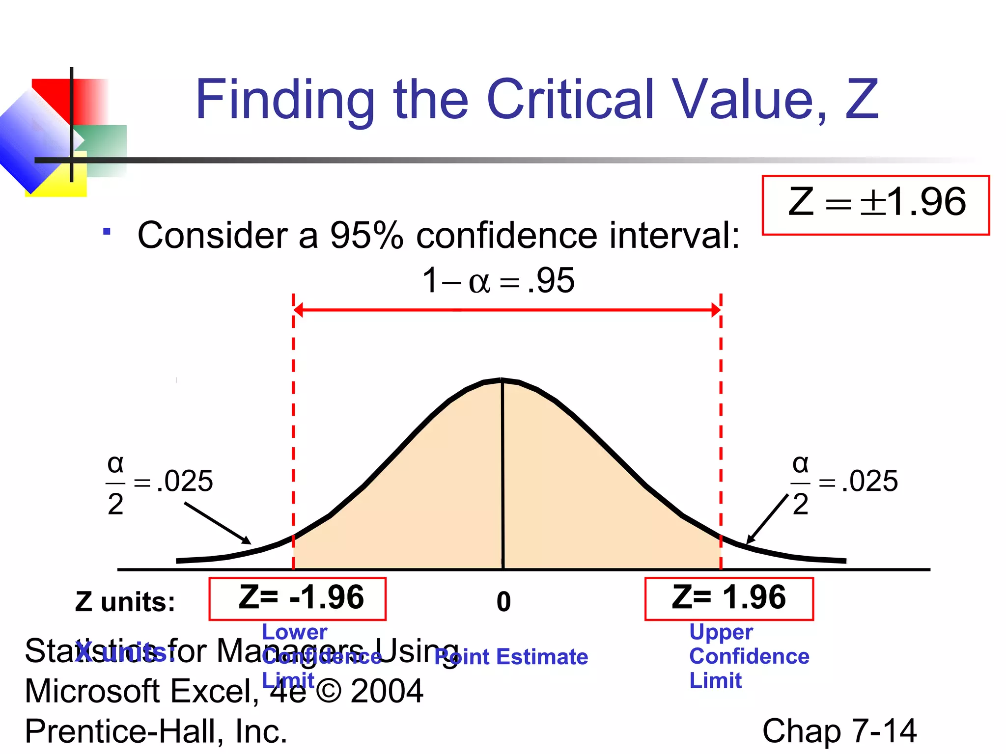
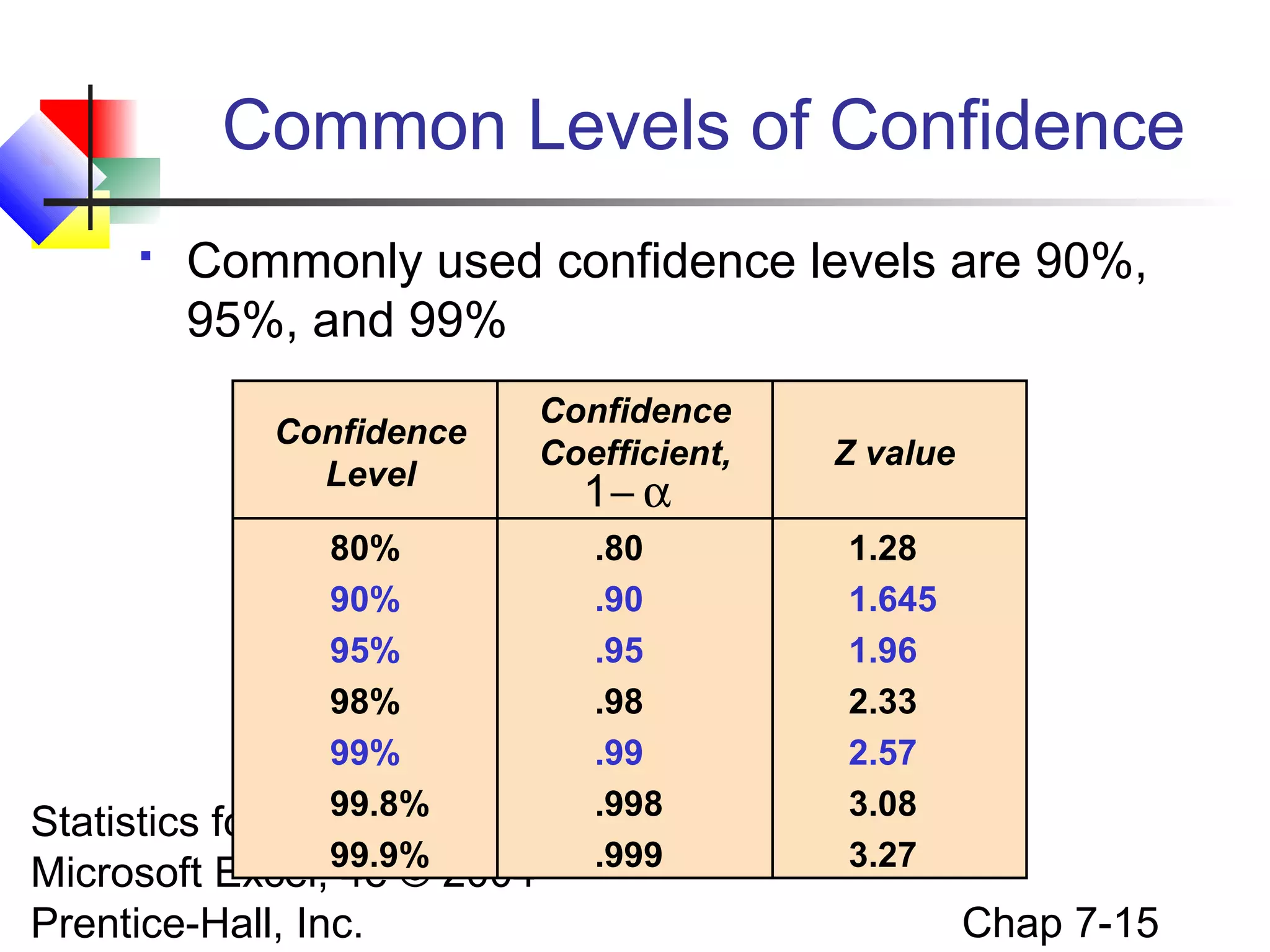
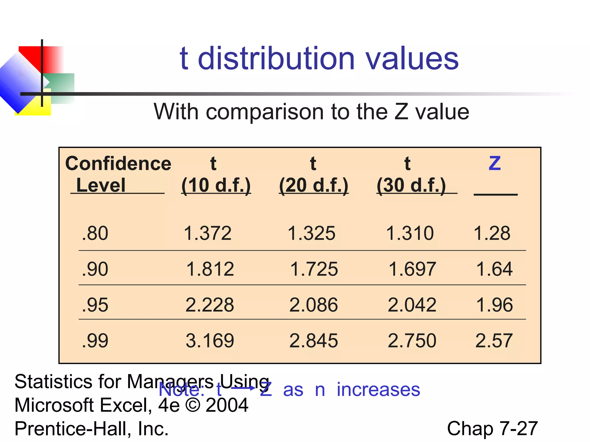
Common confidence levels and corresponding Z values for constructing confidence intervals.
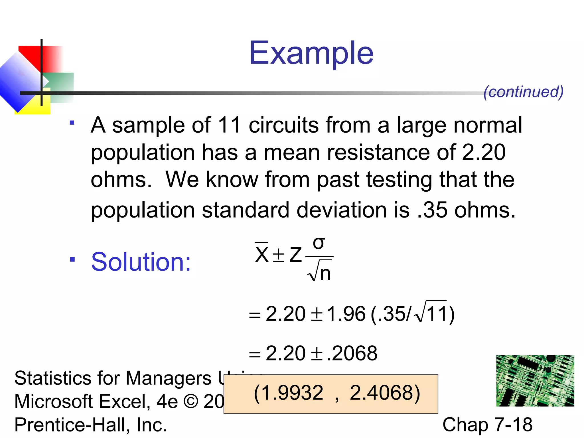
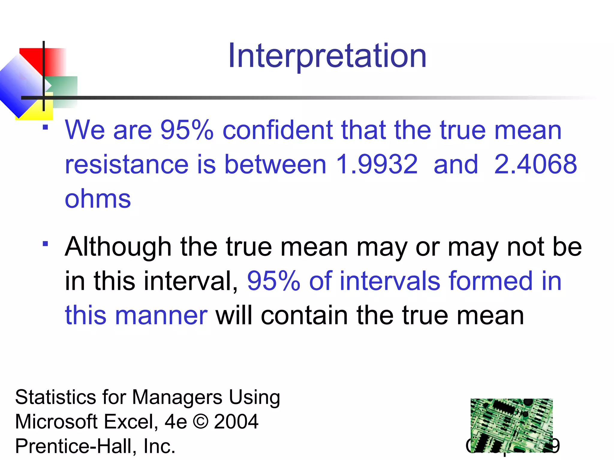
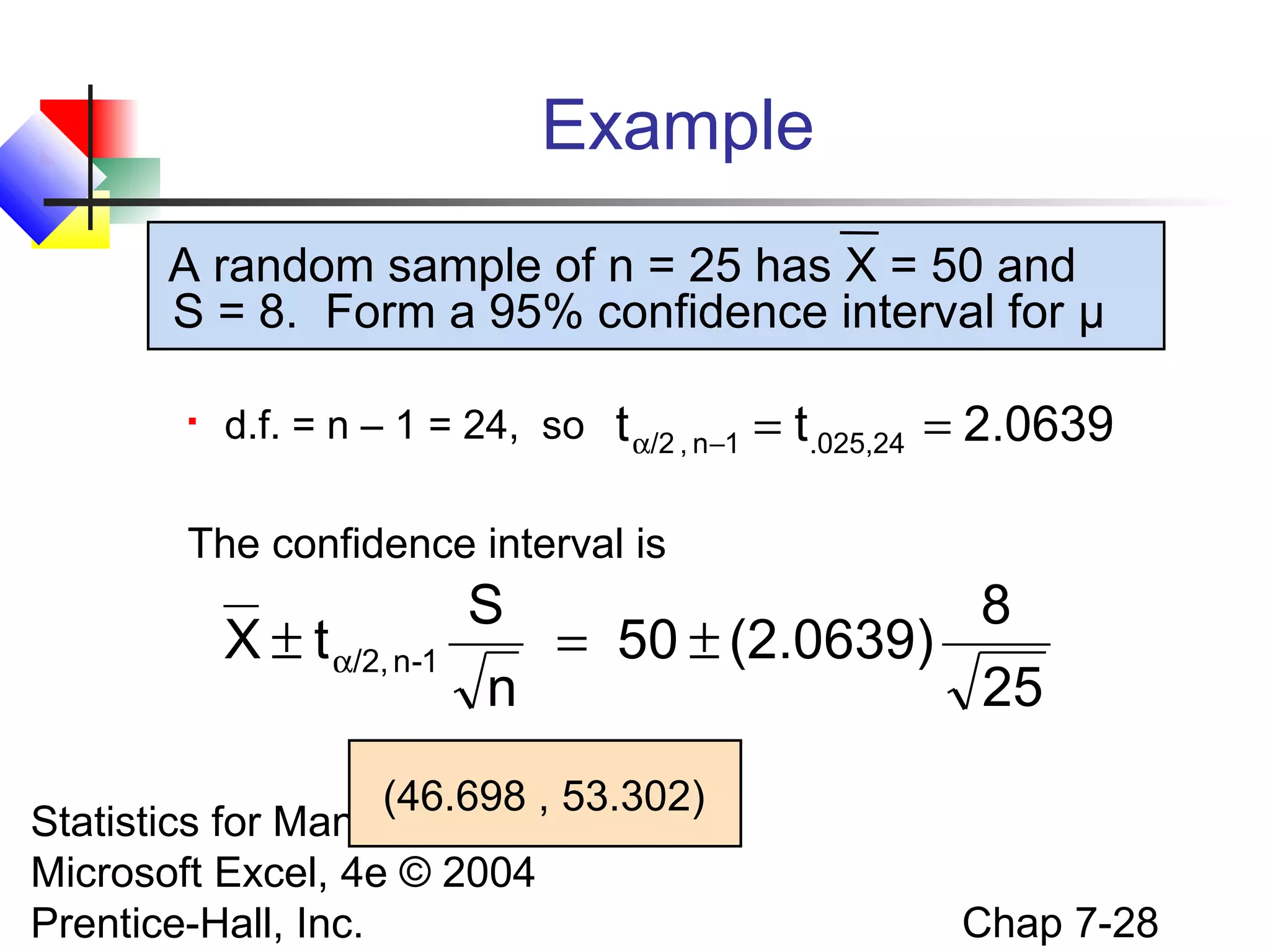
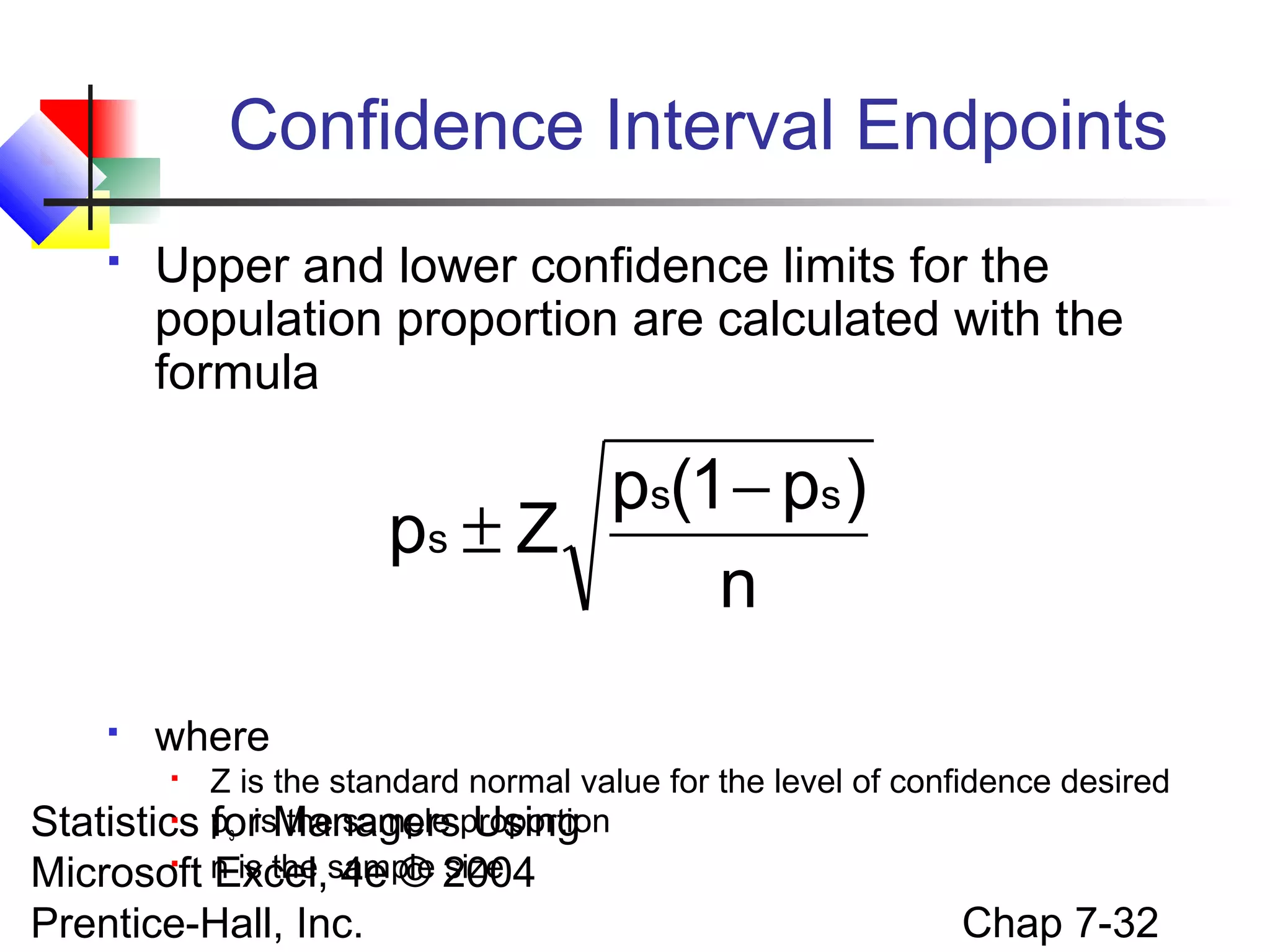
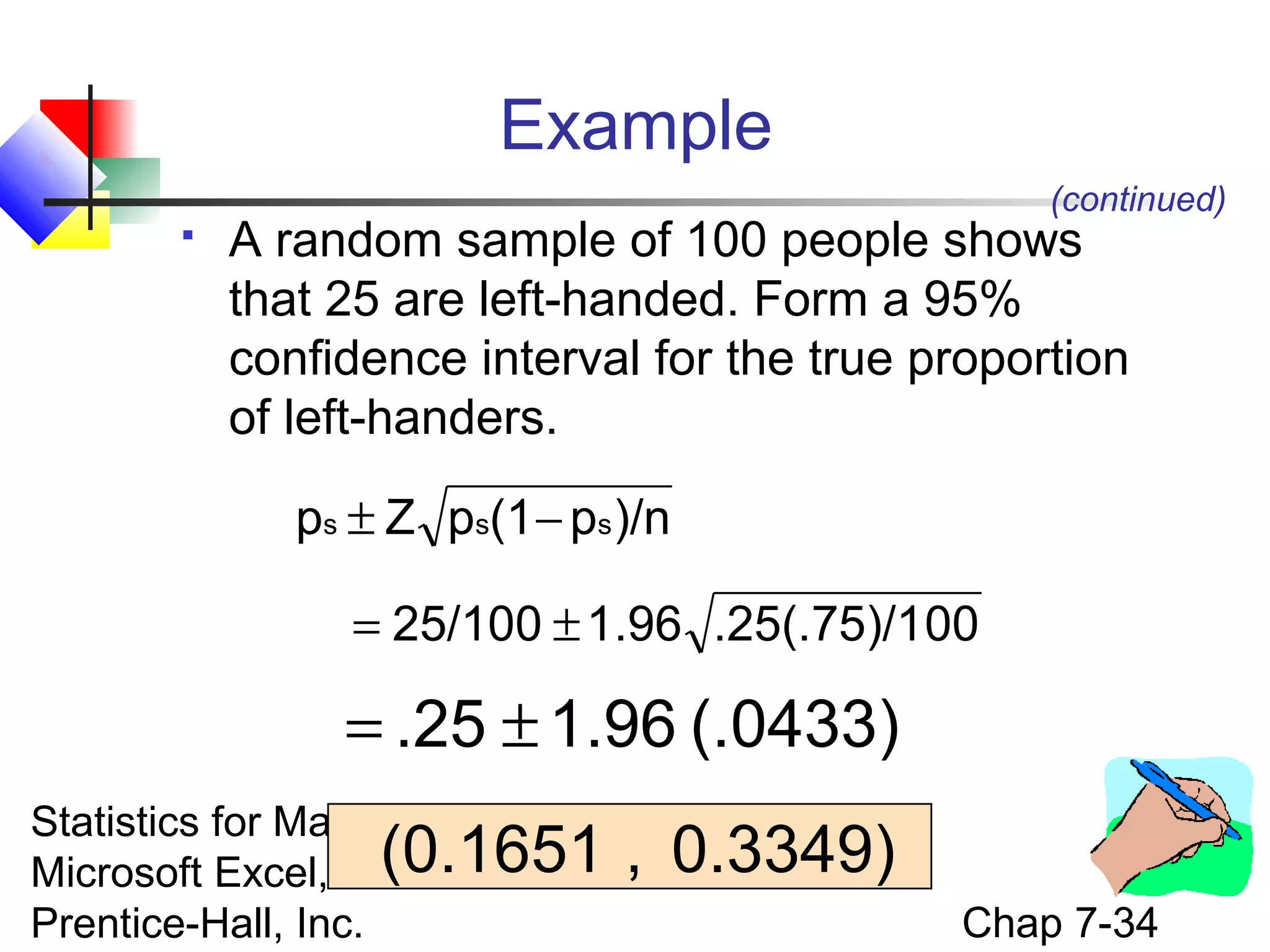
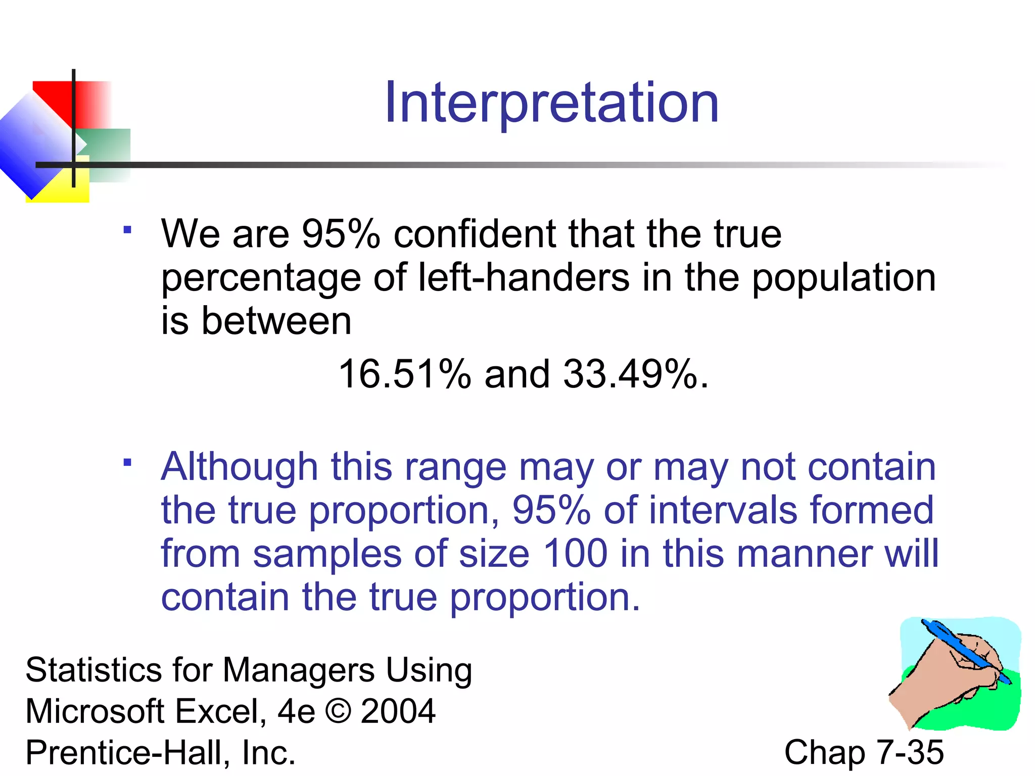
Formulas for determining confidence intervals with examples and interpretation of results.
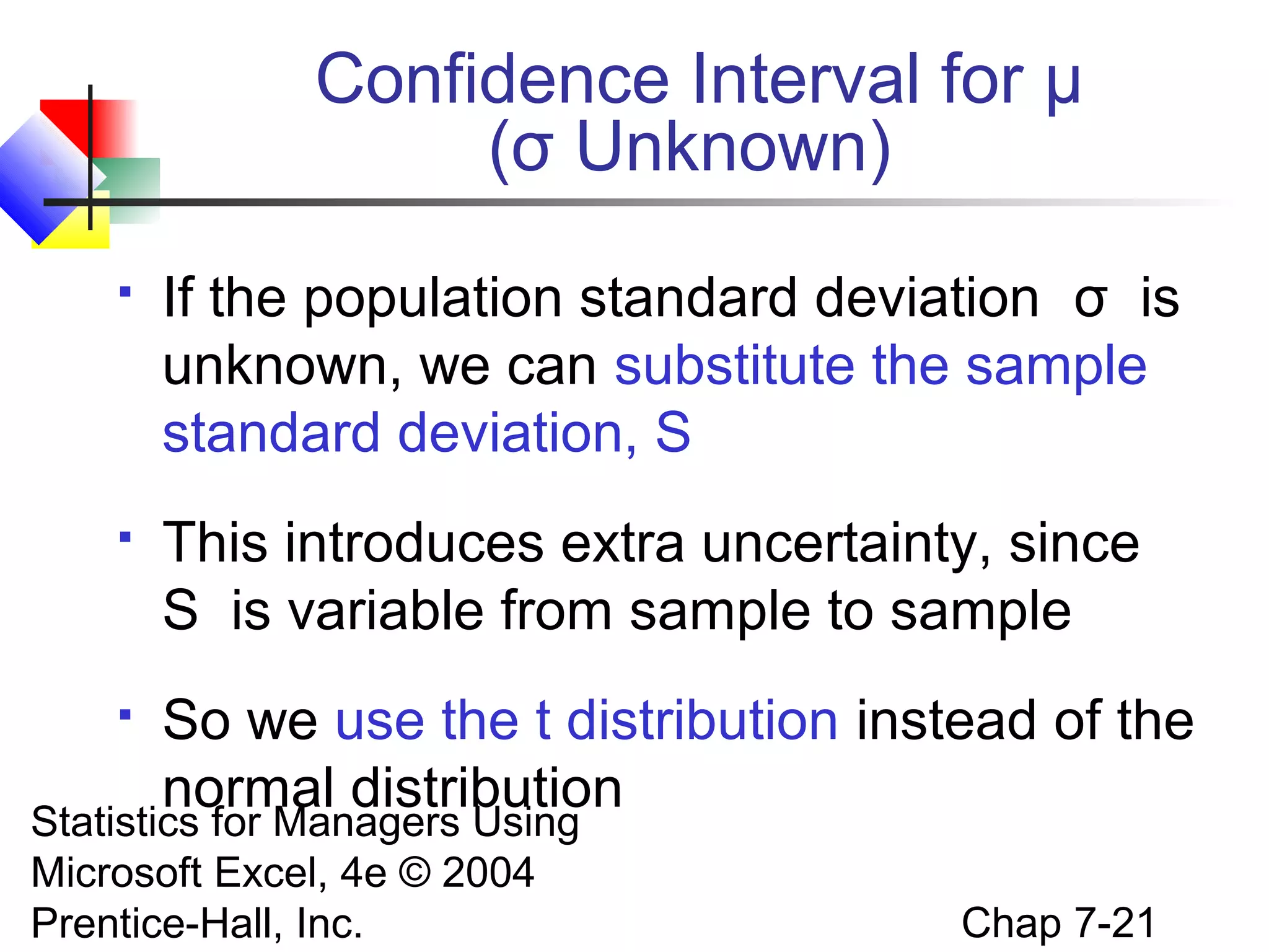
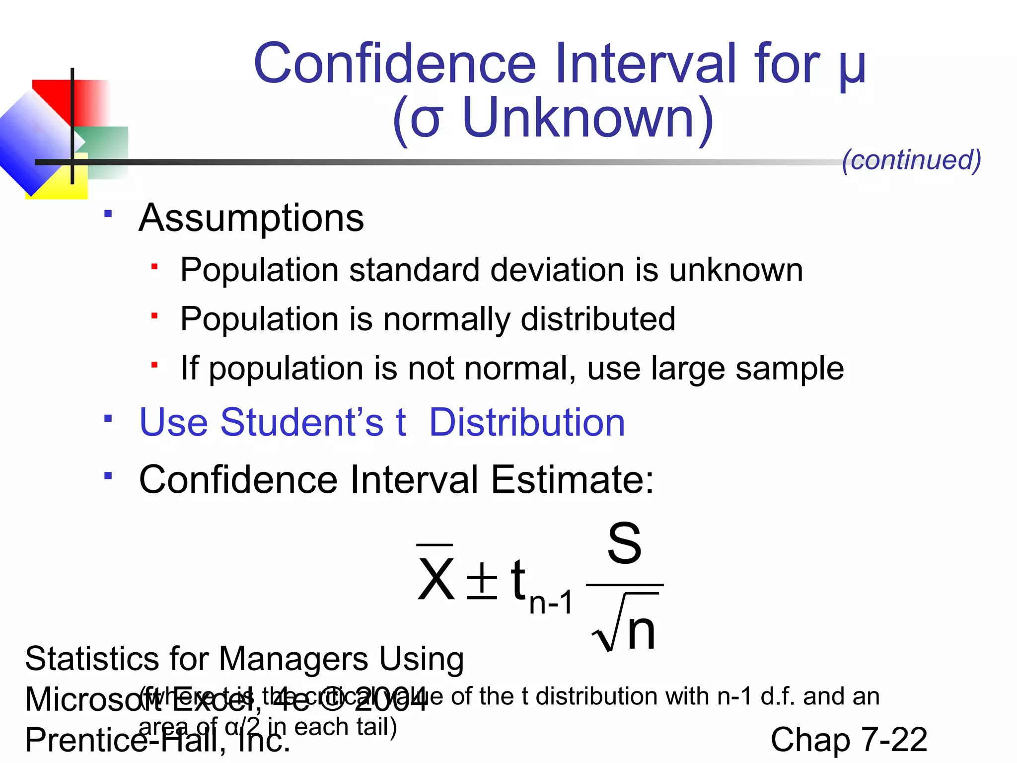
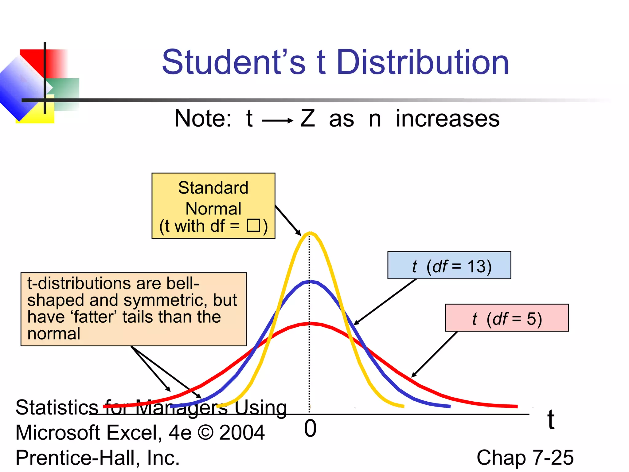
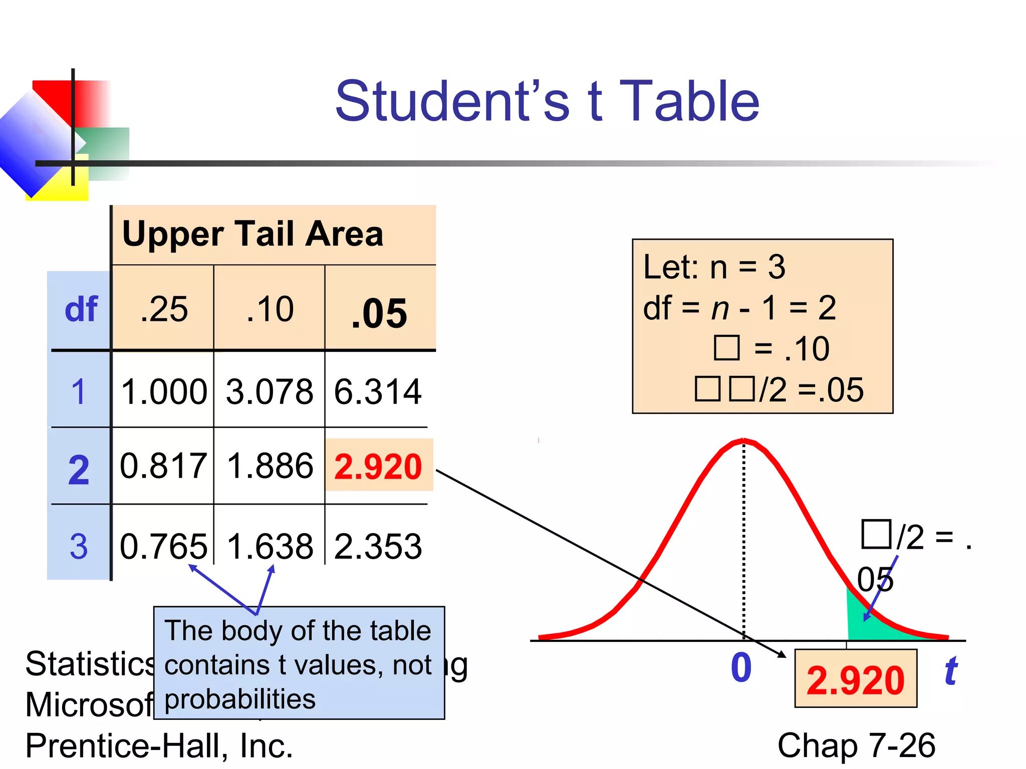
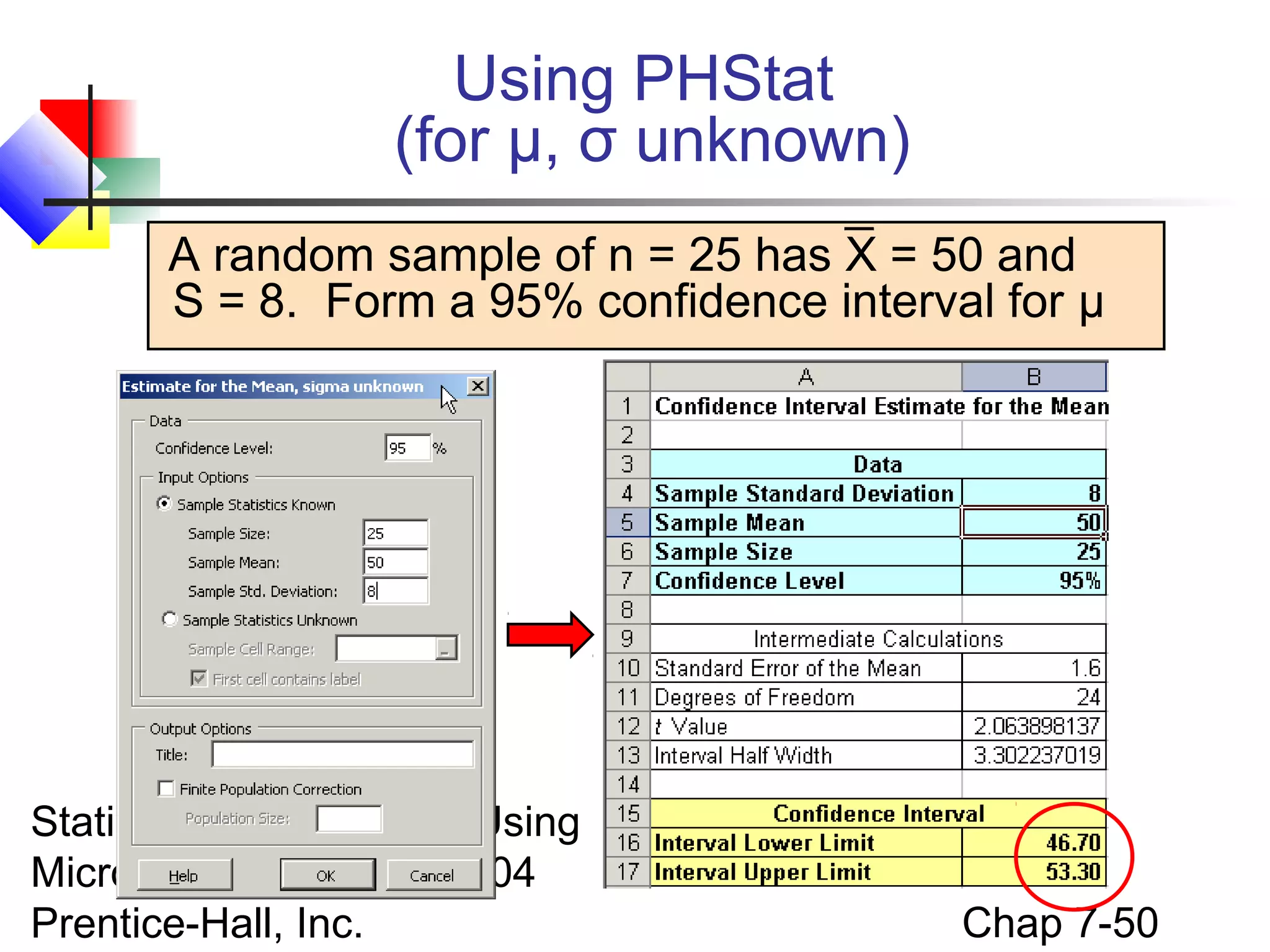
Estimating confidence intervals using t-distribution when population standard deviation is unknown.
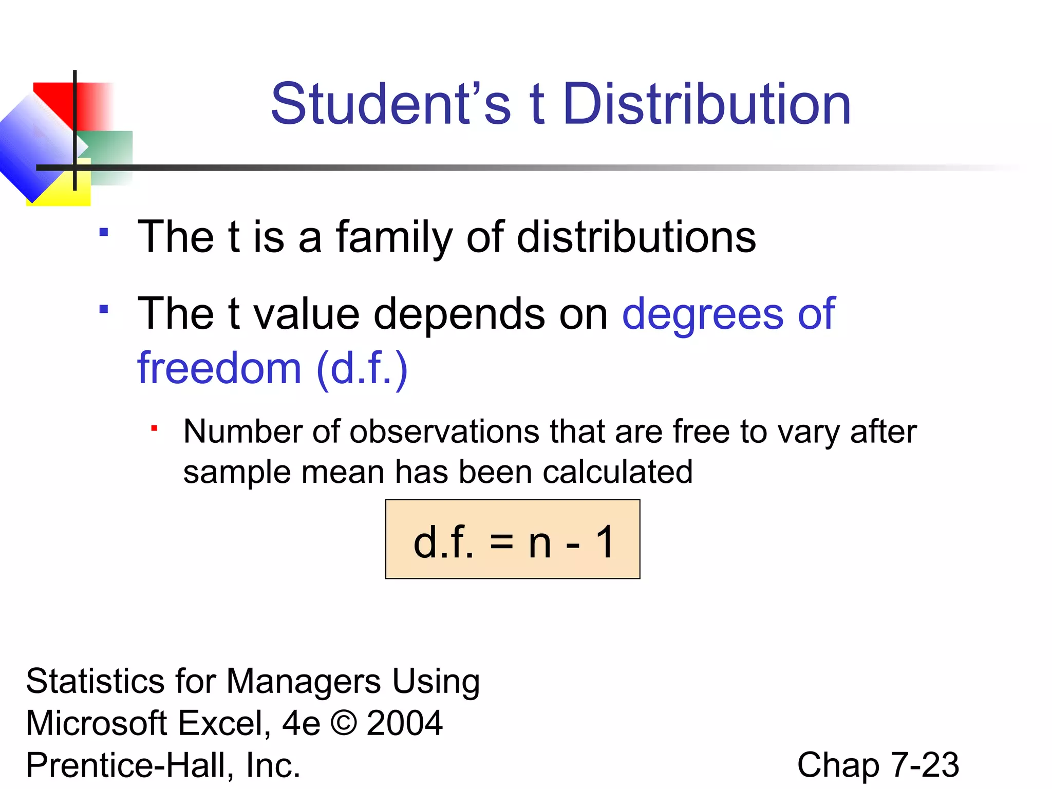
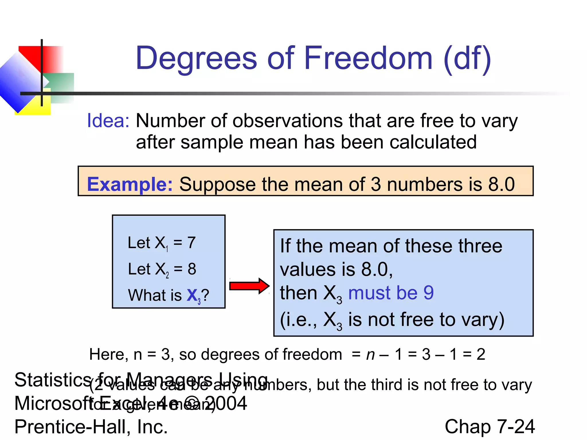
Concept of degrees of freedom in statistical samples and confidence interval estimation.
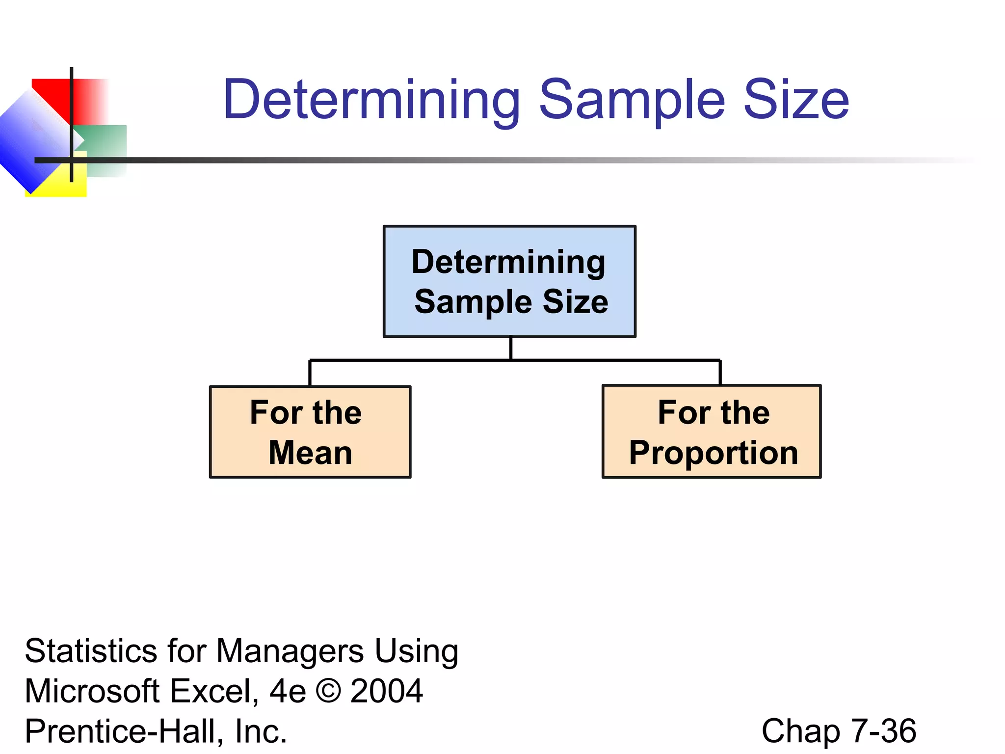
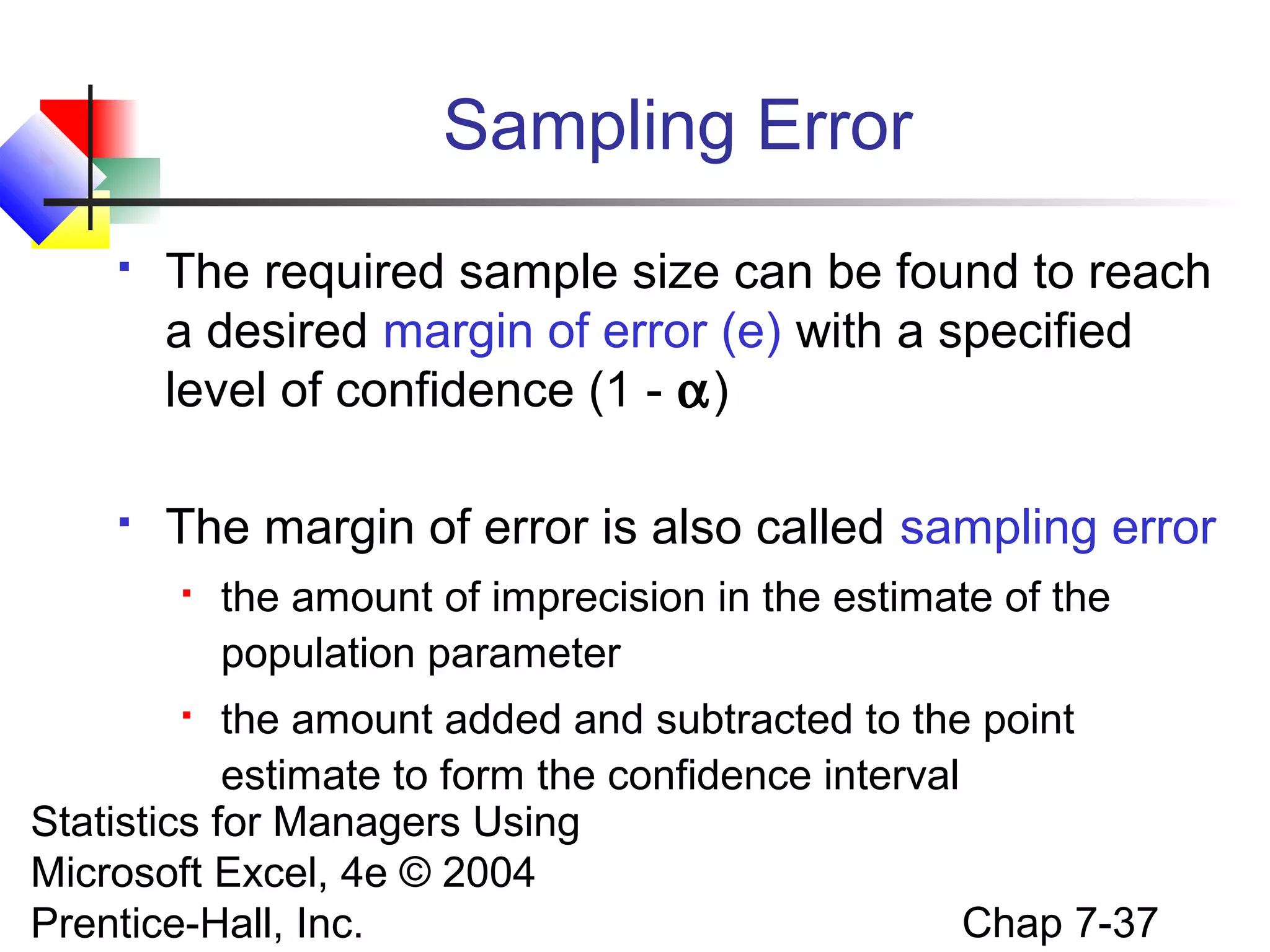
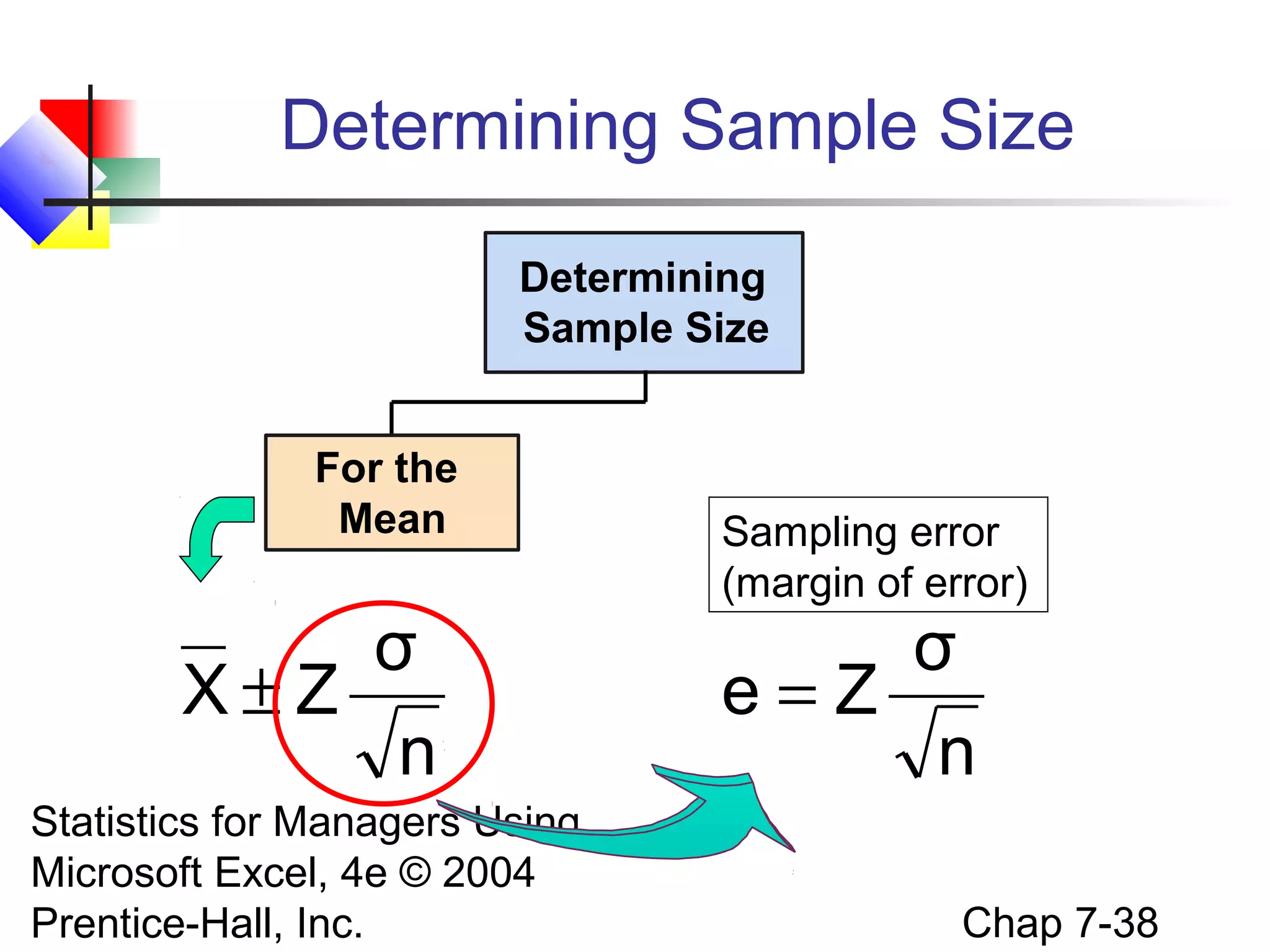
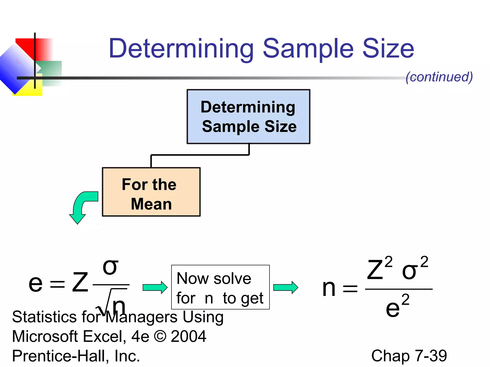
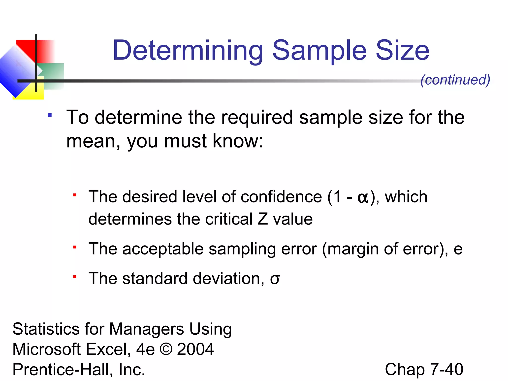
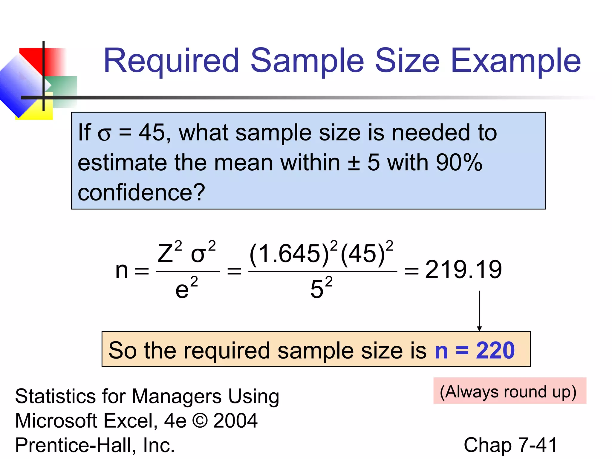
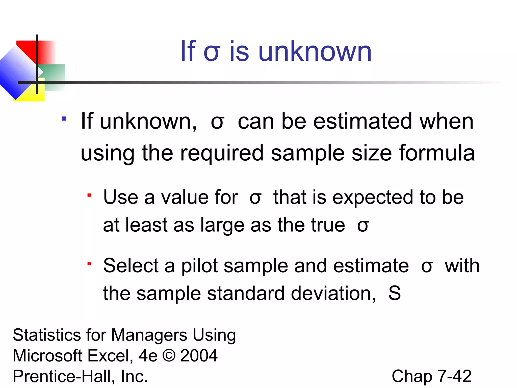
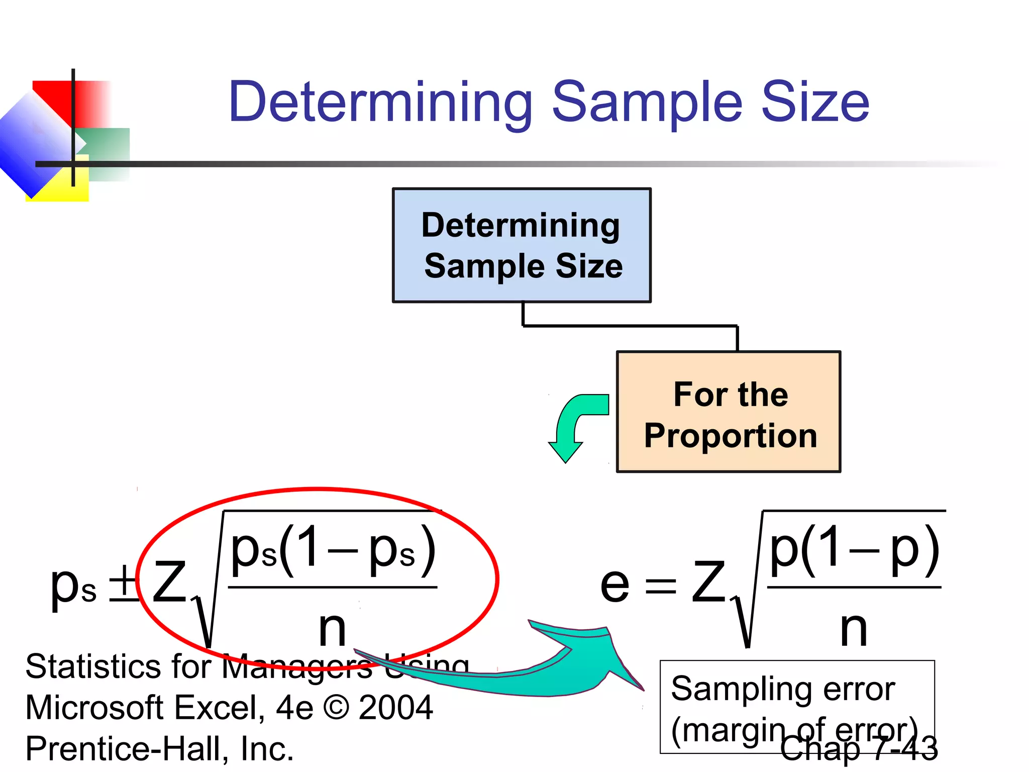
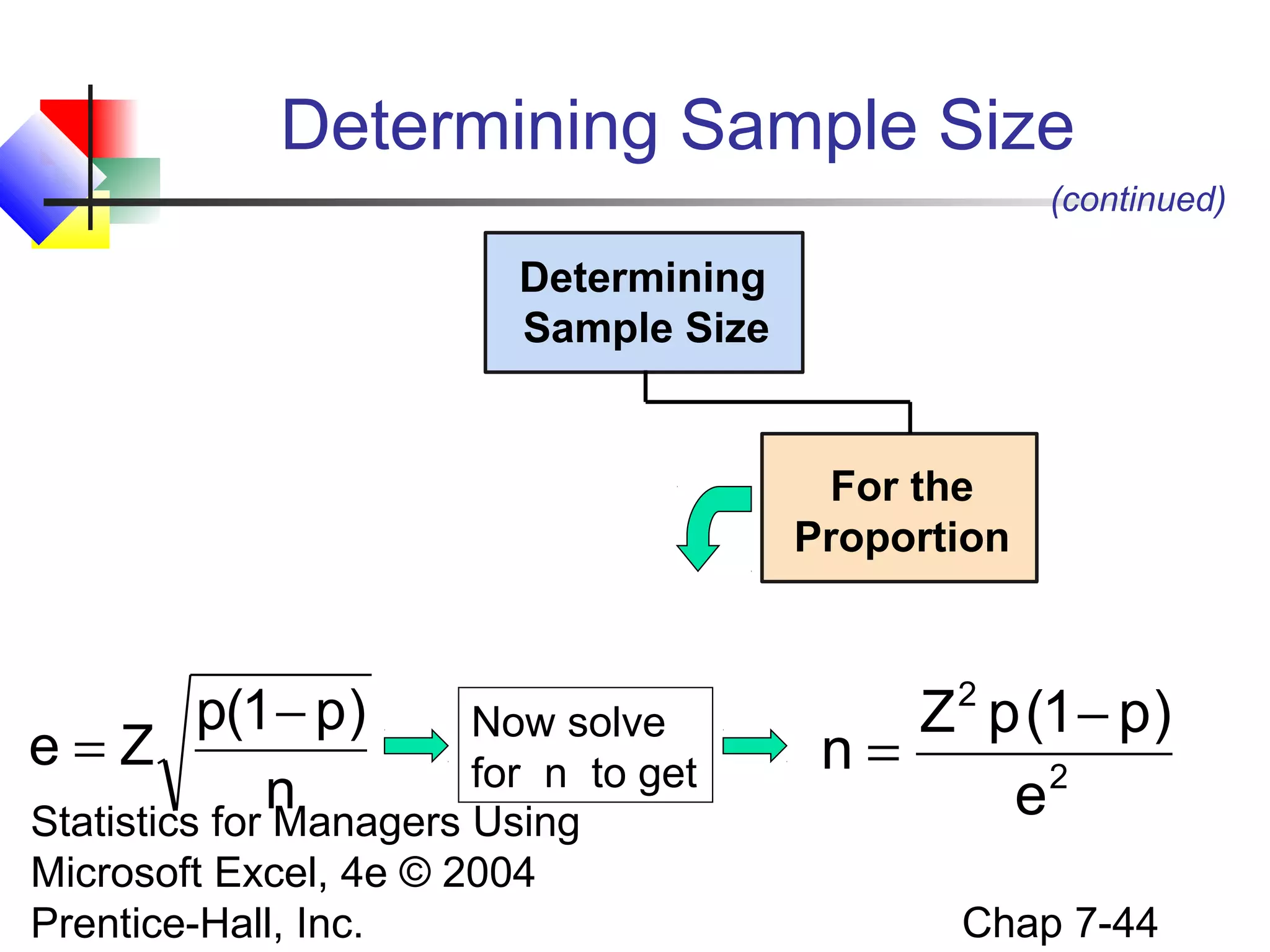
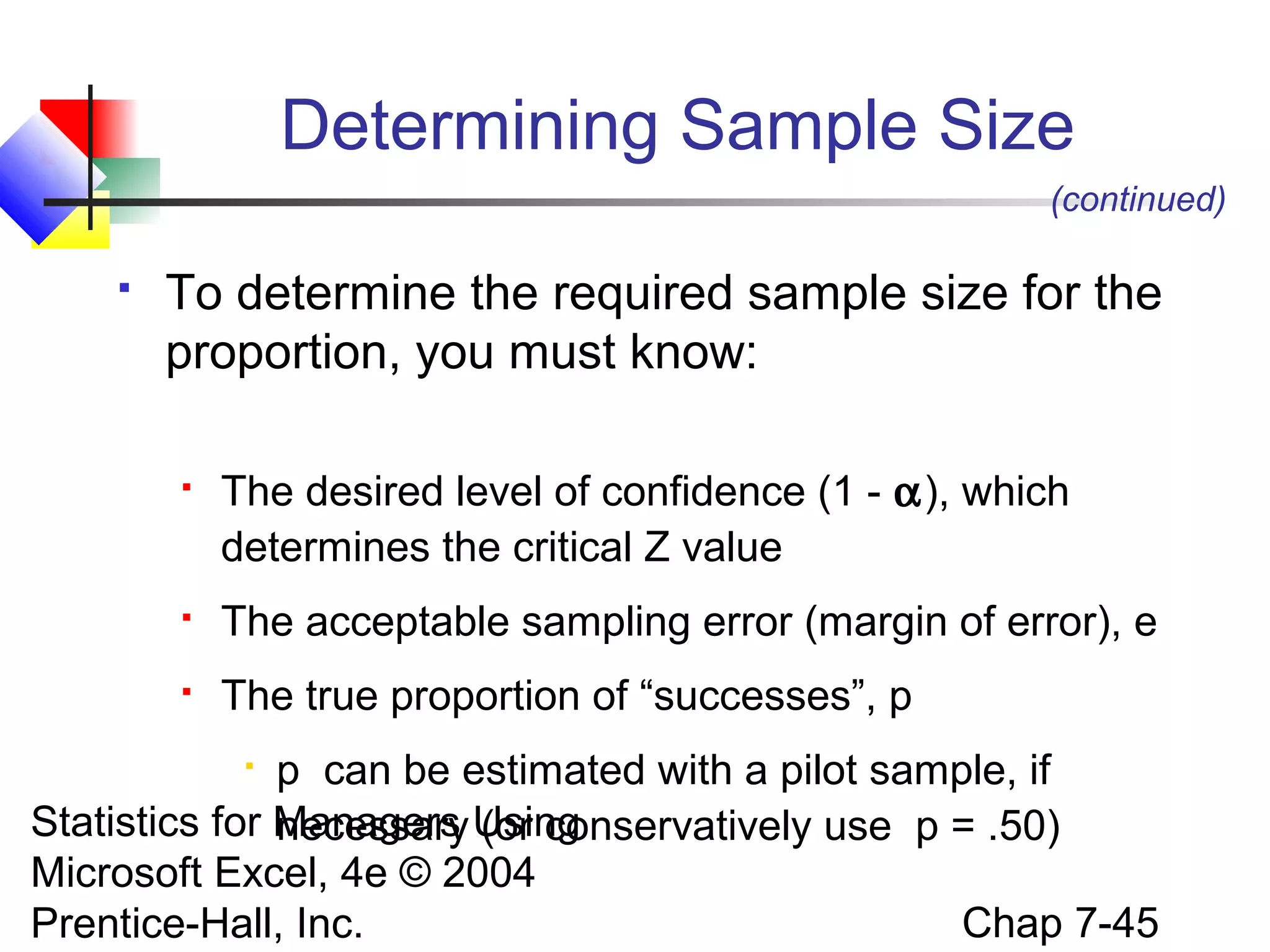
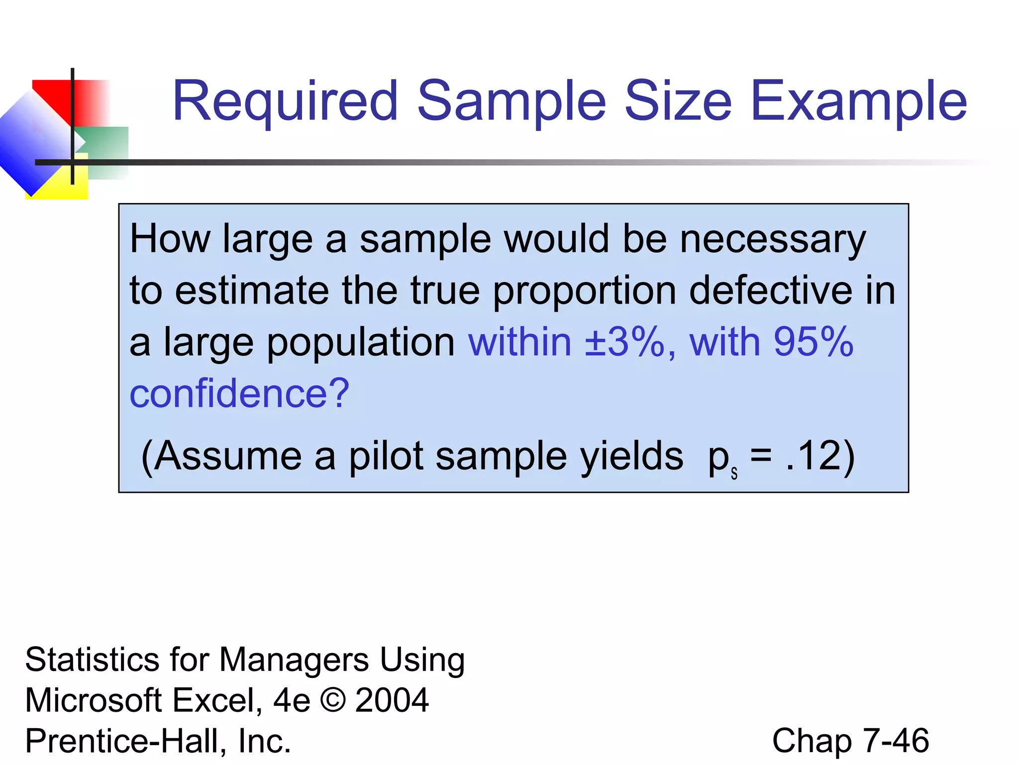
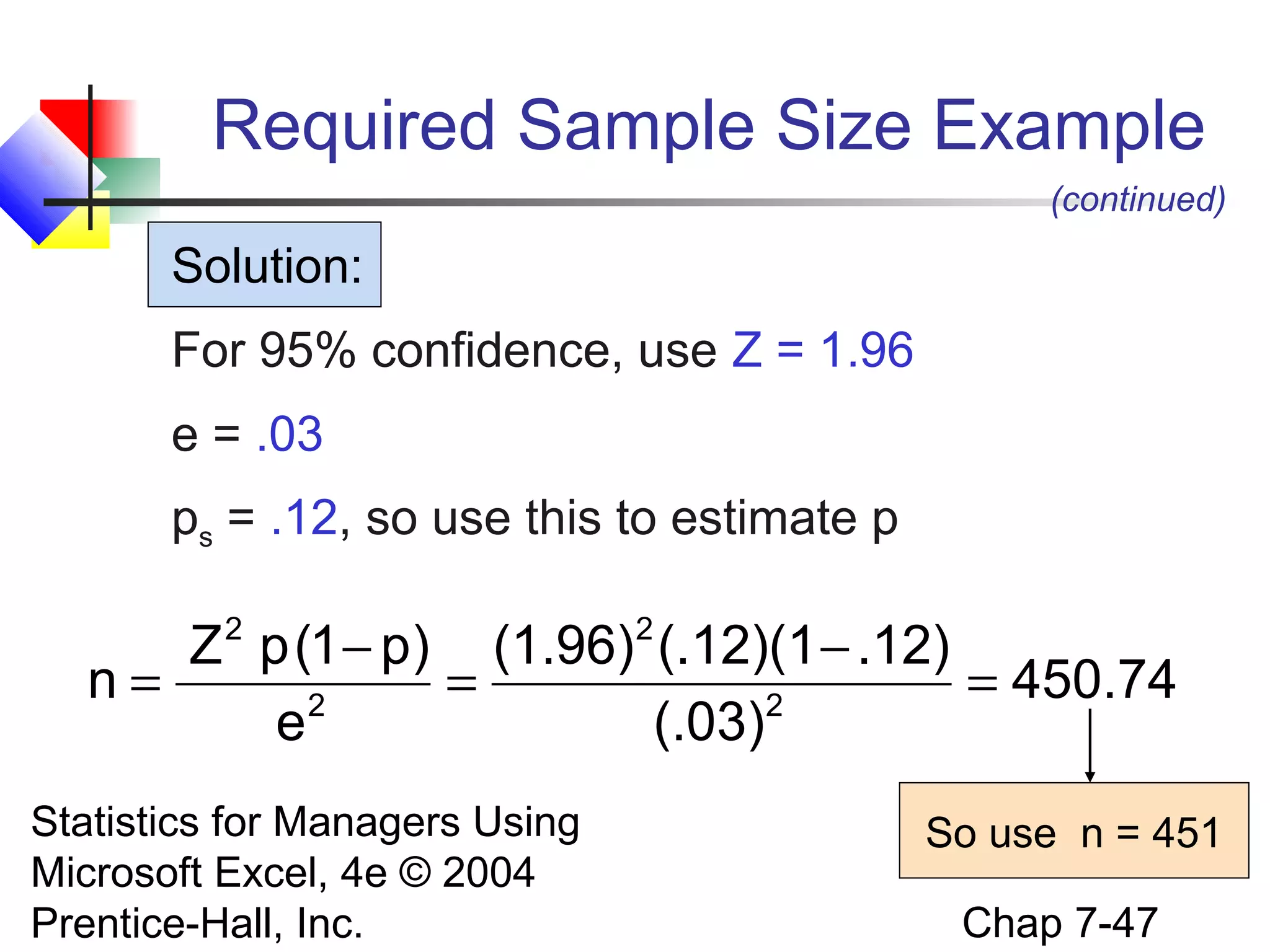
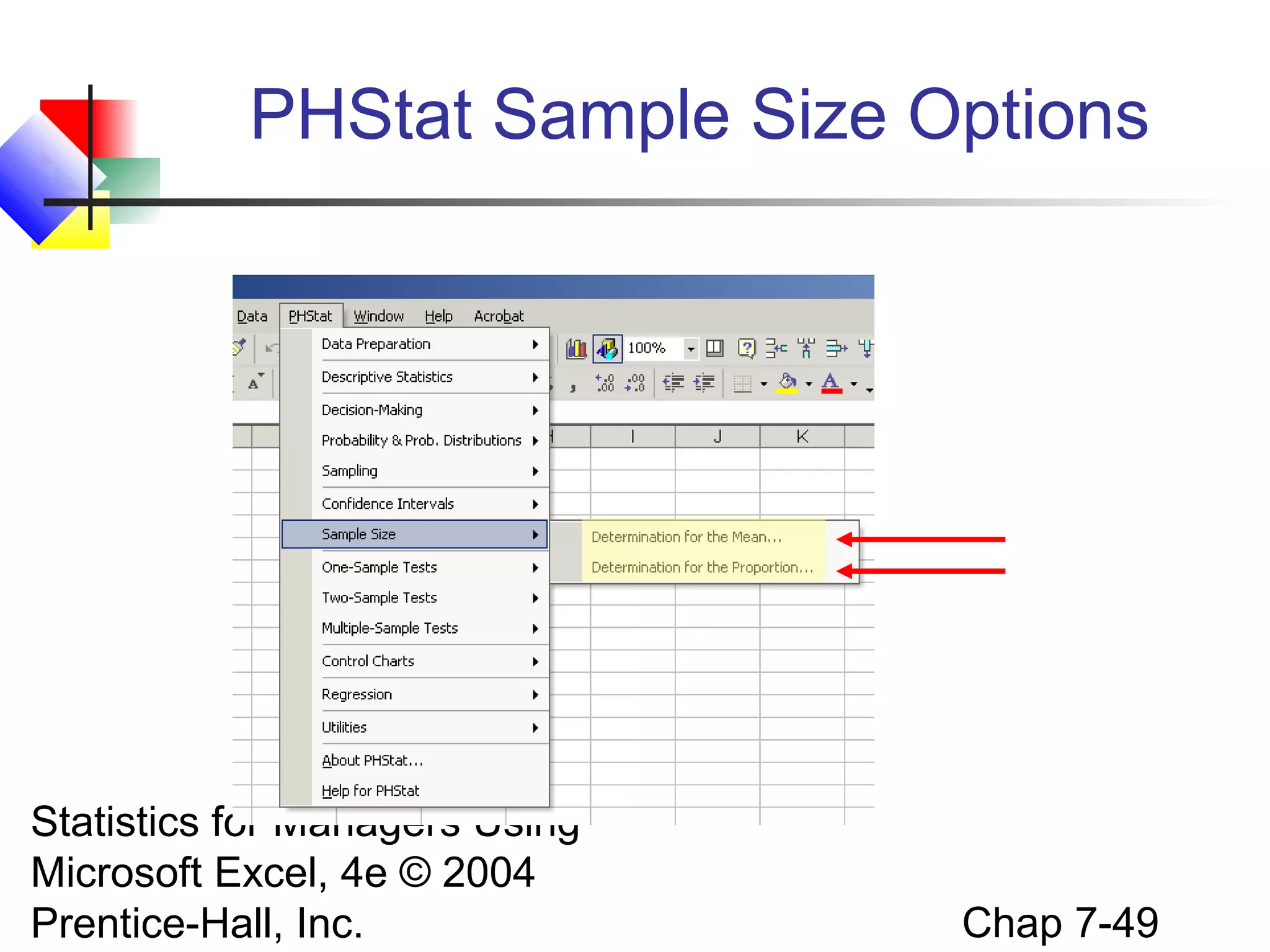
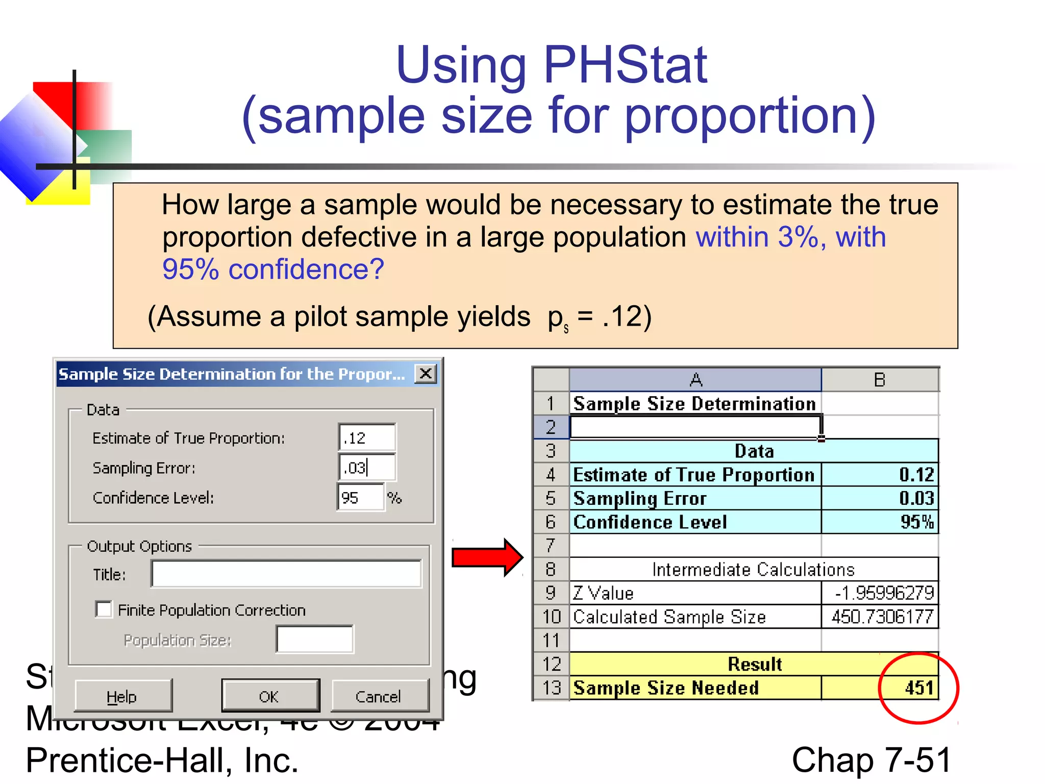
Methodology for determining required sample size for estimates based on confidence levels and margin of error.
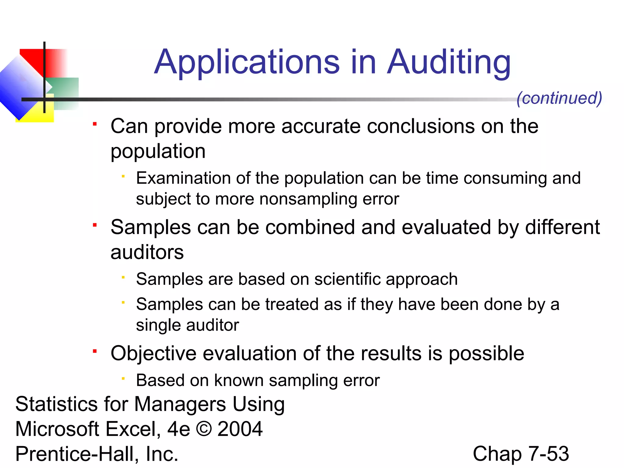
Six advantages of using statistical sampling in auditing for objective and accurate results.
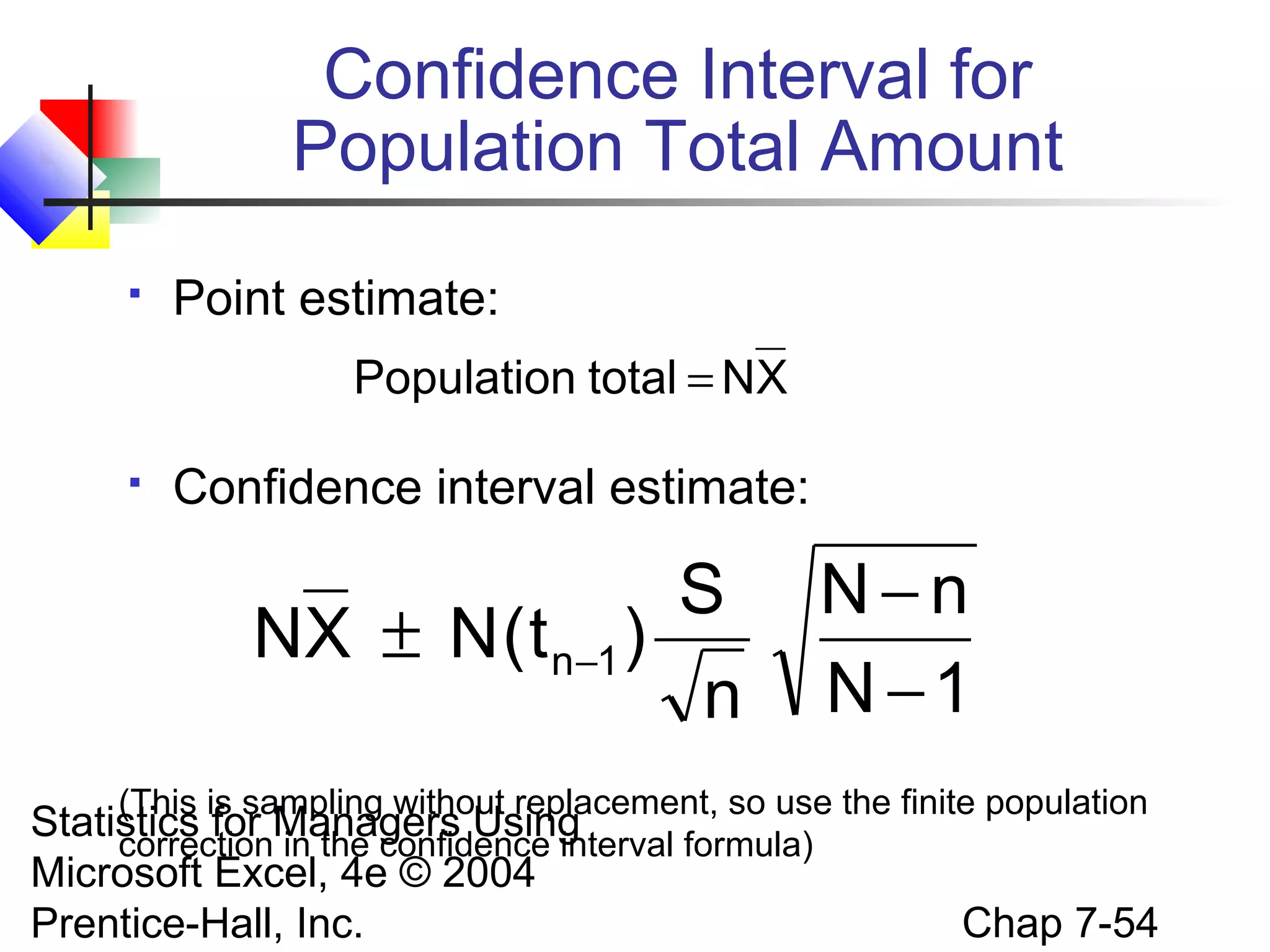
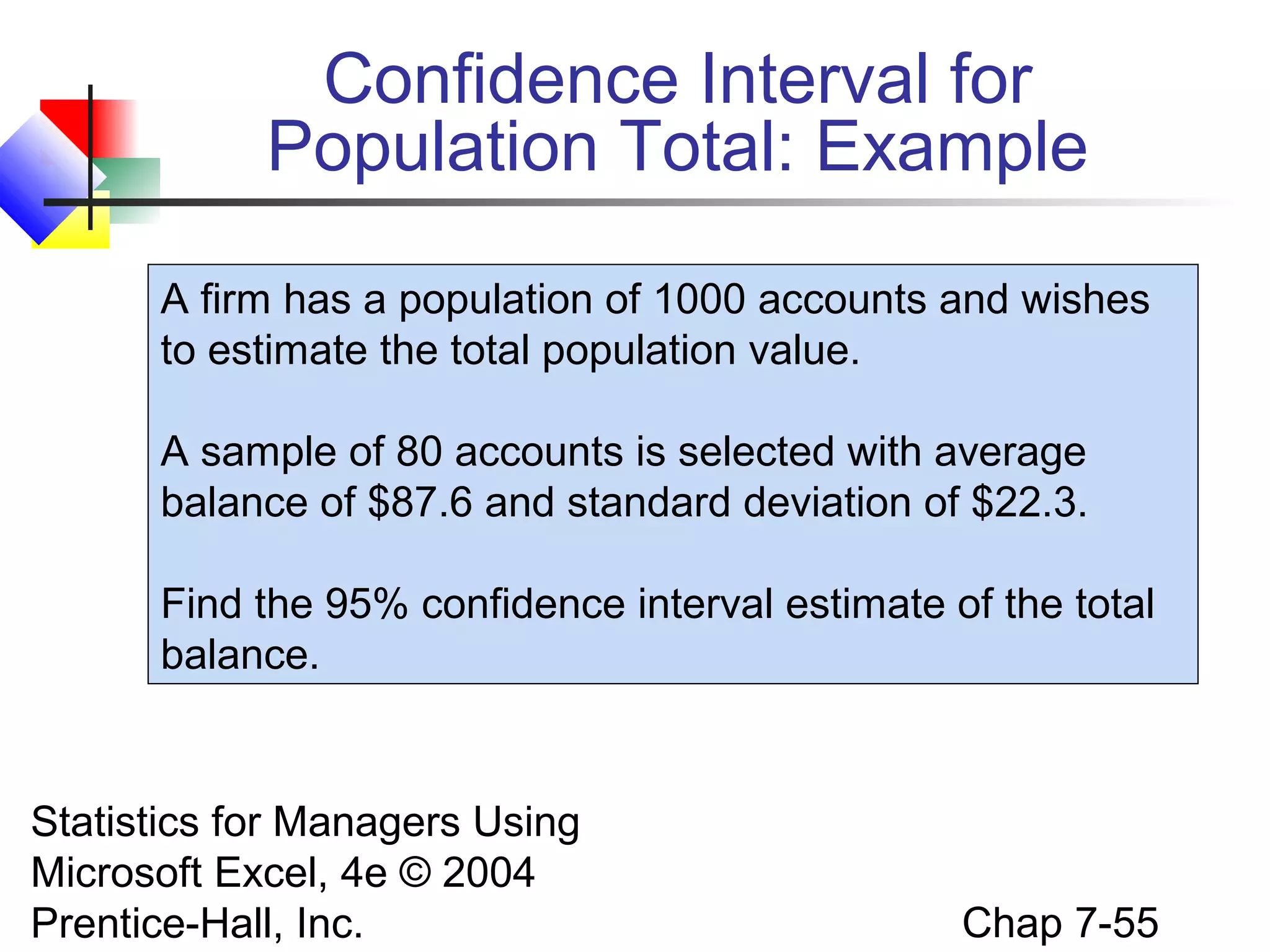
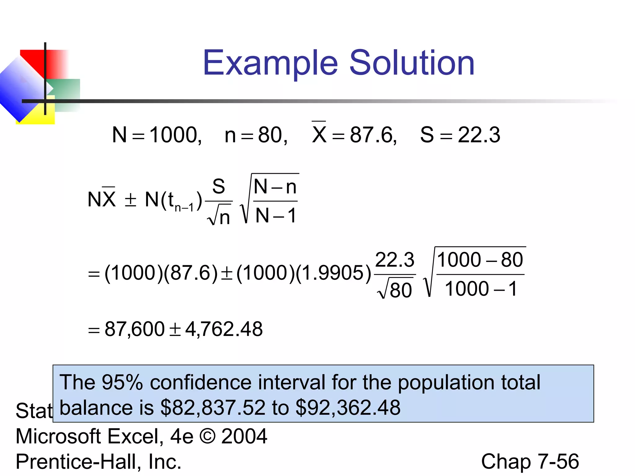
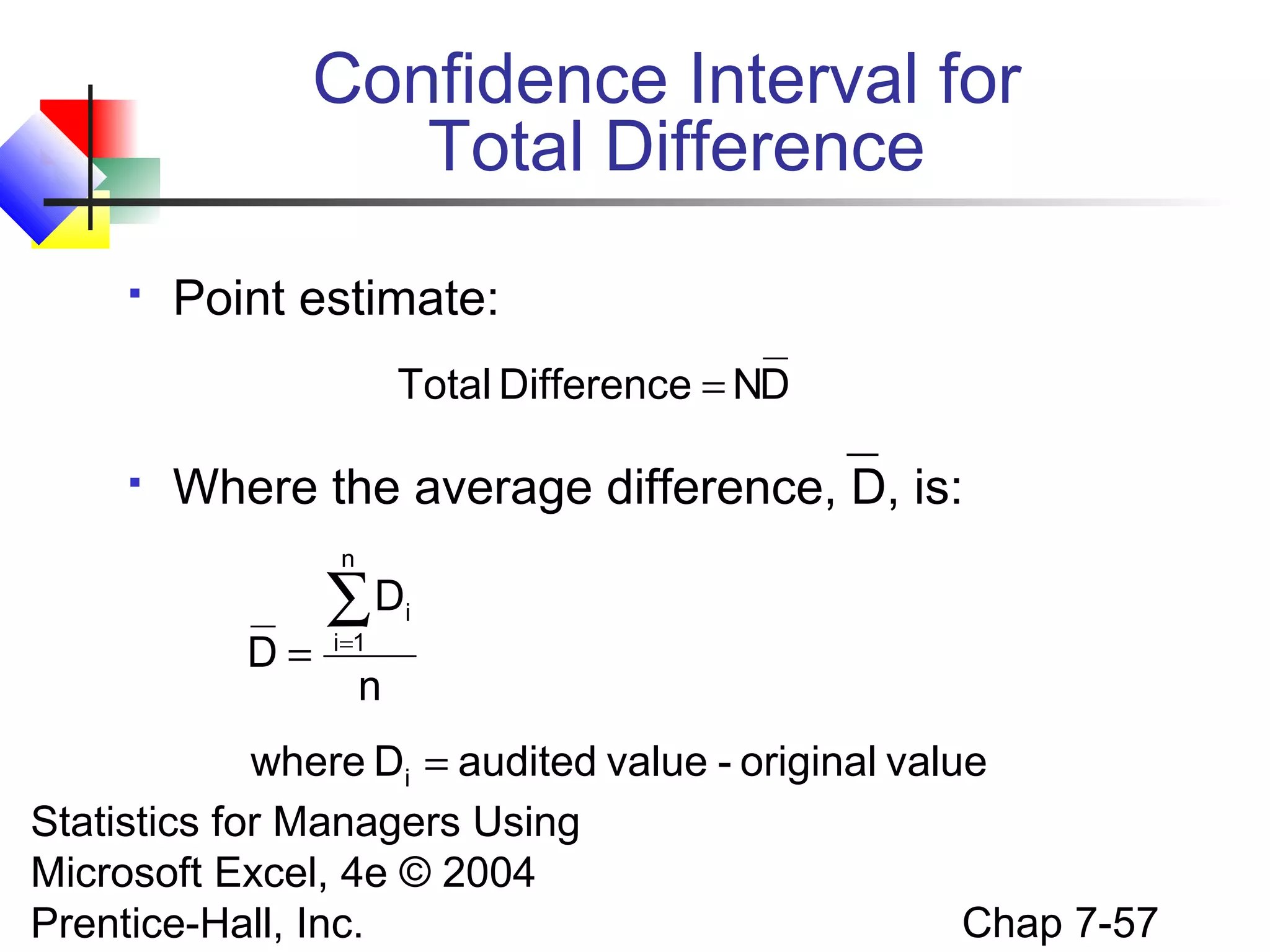
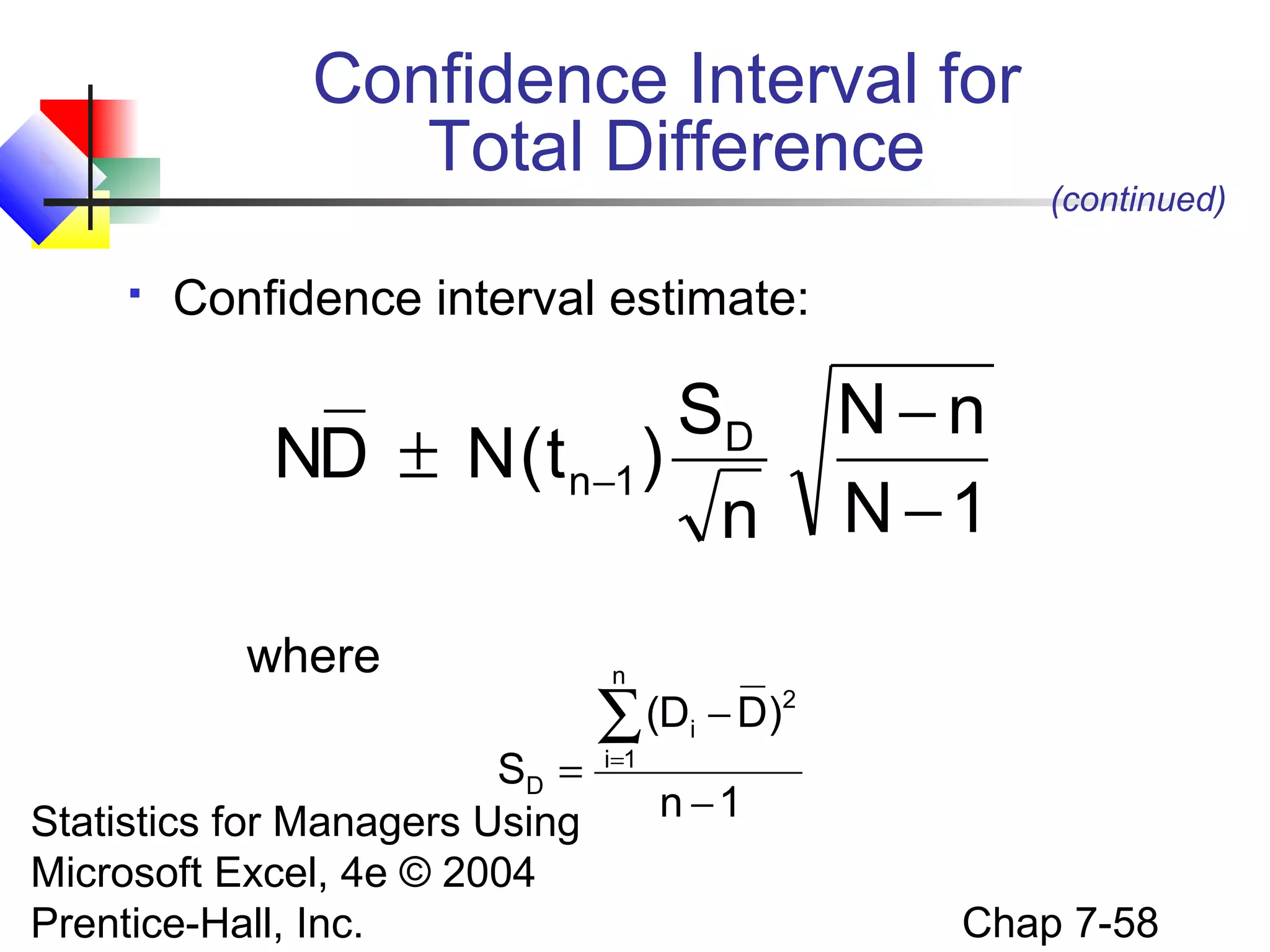
Estimation of total population values and the corresponding confidence interval calculations.
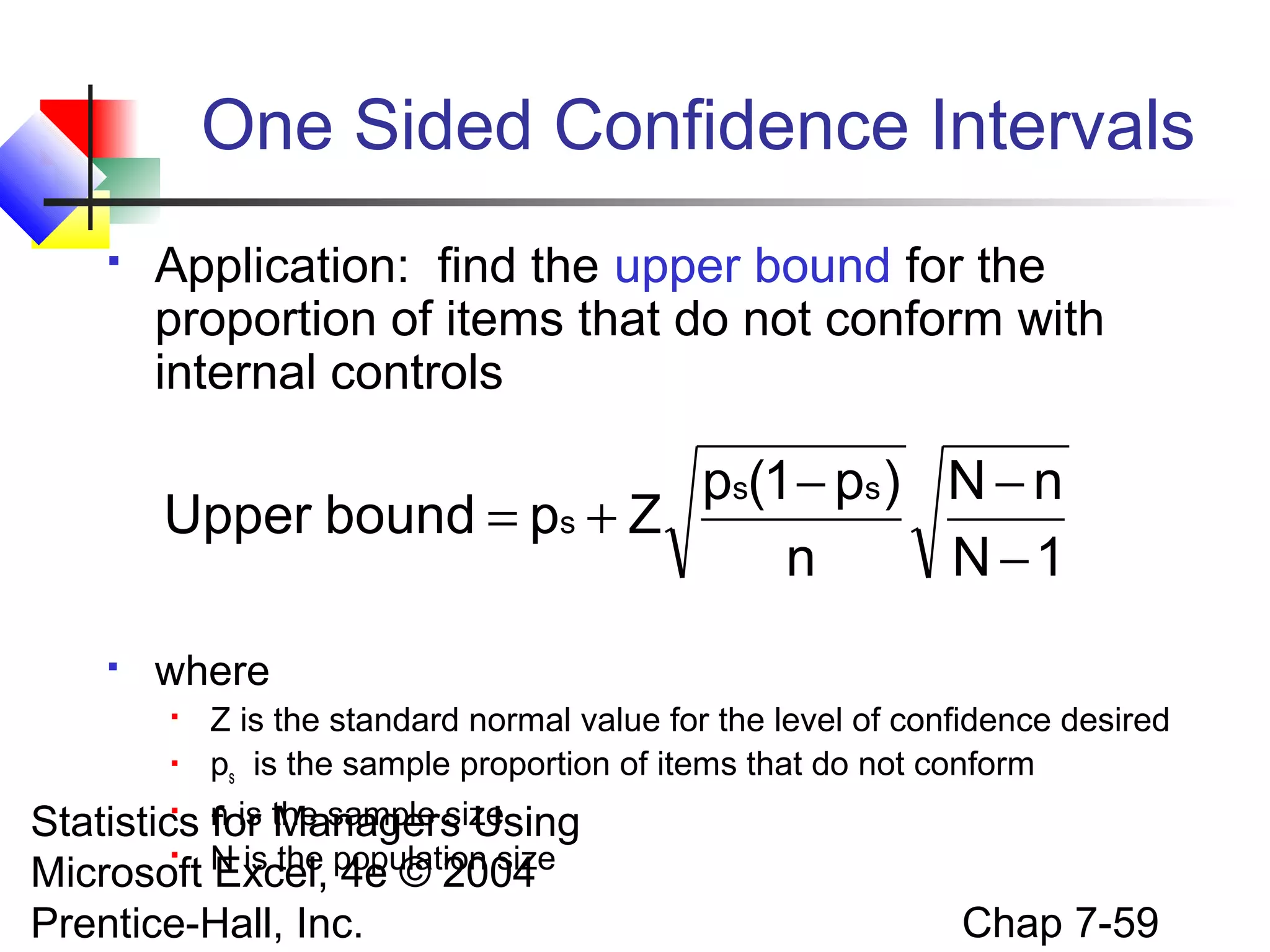
Confidence intervals for total difference, one-sided intervals, ethical considerations.
Recap of key concepts discussed in the chapter including confidence intervals, estimates, and applications.


![Vibe Coding vs. Spec-Driven Development [Free Meetup]](https://cdn.slidesharecdn.com/ss_thumbnails/vibecodingvsspecdrivendevelopment-251209105622-43f455e7-thumbnail.jpg?width=640&height=640&fit=bounds)


