Two Sample Tests

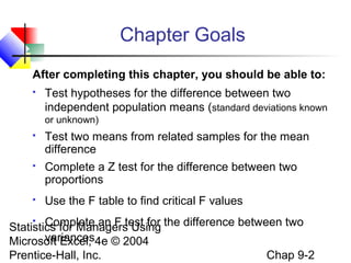
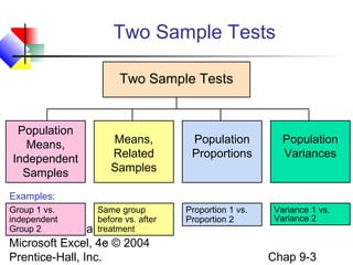
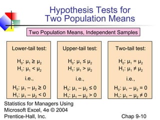
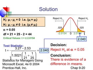
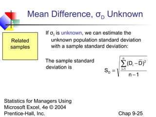
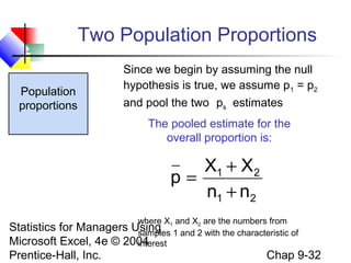
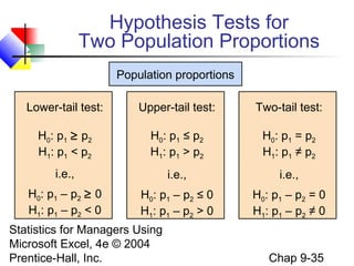
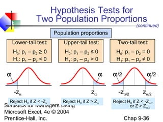
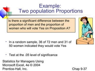
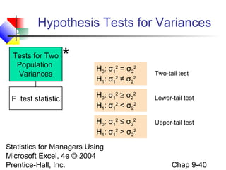
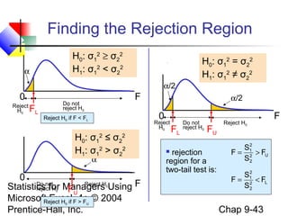
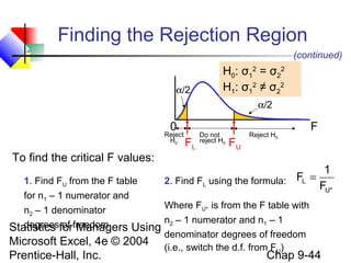
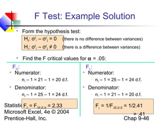
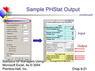
Statistics for Managers Using Microsoft Excel, 4e © 2004 Prentice-Hall, Inc. Chap 9-1
Chapter 9
Two-Sample Tests
Statistics for Managers
Using Microsoft®
Excel
4th
Edition

Statistics for Managers Using
Microsoft Excel, 4e © 2004
Prentice-Hall, Inc. Chap 9-2
Chapter Goals
After completing this chapter, you should be able to:
 Test hypotheses for the difference between two
independent population means (standard deviations known
or unknown)
 Test two means from related samples for the mean
difference
 Complete a Z test for the difference between two
proportions
 Use the F table to find critical F values
 Complete an F test for the difference between two
variances

Two Sample Tests
Two Sample Tests
Population
Means,
Independent
Samples
Means,
Related
Samples
Population
Variances
Group 1 vs.
independent
Group 2
Same group
before vs. after
treatment
Variance 1 vs.
Variance 2
Examples:
Population
Proportions
Proportion 1 vs.
Proportion 2

Difference Between Two Means
Population means,
independent
samples
σ1 and σ2 known
σ1 and σ2 unknown
Goal: Test hypotheses or form
a confidence interval for the
difference between two
population means, μ1 – μ2
The point estimate for the
difference is
X1 – X2
*

Independent Samples
Population means,
independent
samples
 Different data sources
 Unrelated
 Independent

Sample selected from one
population has no effect on
the sample selected from
the other population
 Use the difference between 2
sample means
 Use Z test or pooled variance
t test
*
σ1 and σ2 known
σ1 and σ2 unknown

Difference Between Two Means
Population means,
independent
samples
σ1 and σ2 known
σ1 and σ2 unknown
*
Use a Z test statistic
Use S to estimate unknown
σ , use a t test statistic and
pooled standard deviation

Population means,
independent
samples
σ1 and σ2 known
σ1 and σ2 Known
Assumptions:
 Samples are randomly and
independently drawn
 population distributions are
normal or both sample sizes
are ≥ 30
 Population standard
deviations are known
*
σ1 and σ2 unknown

Population means,
independent
samples
σ1 and σ2 known …and the standard error of
X1 – X2 is
When σ1 and σ2 are known and
both populations are normal or
both sample sizes are at least 30,
the test statistic is a Z-value…
2
2
2
1
2
1
XX
n
σ
n
σ
σ 21
+=−
(continued)
σ1 and σ2 Known
*
σ1 and σ2 unknown

Population means,
independent
samples
σ1 and σ2 known ( ) ( )
2
2
2
1
2
1
2121
n
σ
n
σ
μμXX
Z
+
−−−
=
The test statistic for
μ1 – μ2 is:
σ1 and σ2 Known
*
σ1 and σ2 unknown
(continued)

Hypothesis Tests for
Two Population Means
Lower-tail test:
H0: μ1 ≥ μ2
H1: μ1 < μ2
i.e.,
H0: μ1 – μ2 ≥ 0
H1: μ1 – μ2 < 0
Upper-tail test:
H0: μ1 ≤ μ2
H1: μ1 > μ2
i.e.,
H0: μ1 – μ2 ≤ 0
H1: μ1 – μ2 > 0
Two-tail test:
H0: μ1 = μ2
H1: μ1 ≠ μ2
i.e.,
H0: μ1 – μ2 = 0
H1: μ1 – μ2 ≠ 0
Two Population Means, Independent Samples

Two Population Means, Independent Samples
Lower-tail test:
H0: μ1 – μ2 ≥ 0
H1: μ1 – μ2 < 0
Upper-tail test:
H0: μ1 – μ2 ≤ 0
H1: μ1 – μ2 > 0
Two-tail test:
H0: μ1 – μ2 = 0
H1: μ1 – μ2 ≠ 0
α α/2 α/2α
-zα -zα/2zα zα/2
Reject H0 if Z < -Zα Reject H0 if Z > Zα Reject H0 if Z < -Zα/2
or Z > Zα/2
Hypothesis tests for μ1 – μ2

Population means,
independent
samples
σ1 and σ2 known
( )
2
2
2
1
2
1
21
n
σ
n
σ
ZXX +±−
The confidence interval for
μ1 – μ2 is:
Confidence Interval,
σ1 and σ2 Known
*
σ1 and σ2 unknown

Population means,
independent
samples
σ1 and σ2 known
σ1 and σ2 Unknown
Assumptions:
 Samples are randomly and
independently drawn
 Populations are normally
distributed or both sample
sizes are at least 30
 Population variances are
unknown but assumed equal
*σ1 and σ2 unknown

Population means,
independent
samples
σ1 and σ2 known
σ1 and σ2 Unknown
(continued)
Forming interval
estimates:
 The population variances
are assumed equal, so use
the two sample standard
deviations and pool them to
estimate σ
 the test statistic is a t value
with (n1 + n2 – 2) degrees
of freedom

Population means,
independent
samples
σ1 and σ2 known
σ1 and σ2 Unknown
The pooled standard
deviation is
(continued)
( ) ( )
1)n()1(n
S1nS1n
S
21
2
22
2
11
p
−+−
−+−
=*σ1 and σ2 unknown

Population means,
independent
samples
σ1 and σ2 known
σ1 and σ2 Unknown
Where t has (n1 + n2 – 2) d.f.,
and
( ) ( )






+
−−−
=
21
2
p
2121
n
1
n
1
S
μμXX
t
μ1 – μ2 is:
( ) ( )
1)n()1(n
S1nS1n
S
21
2
22
2
112
p
−+−
−+−
=
(continued)

Population means,
independent
samples
σ1 and σ2 known
( ) 





+±− +
21
2
p2-nn21
n
1
n
1
StXX 21
μ1 – μ2 is:
Where
( ) ( )
1)n()1(n
S1nS1n
S
21
2
22
2
112
p
−+−
−+−
=
Confidence Interval,
σ1 and σ2 Unknown

Pooled Sp t Test: Example
You are a financial analyst for a brokerage firm. Is there
a difference in dividend yield between stocks listed on the
NYSE & NASDAQ? You collect the following data:
NYSE NASDAQ
Number 21 25
Sample mean 3.27 2.53
Sample std dev 1.30 1.16
Assuming both populations are
approximately normal with
equal variances, is
there a difference in average
yield (α = 0.05)?

Calculating the Test Statistic
( ) ( ) ( ) ( ) 1.5021
1)25(1)-(21
1.161251.30121
1)n()1(n
S1nS1n
S
22
21
2
22
2
112
p =
−+
−+−
=
−+−
−+−
=
( ) ( ) ( ) 2.040
25
1
21
1
5021.1
02.533.27
n
1
n
1
S
μμXX
t
21
2
p
2121
=






+
−−
=






+
−−−
=
The test statistic is:

Solution
H0: μ1 - μ2 = 0 i.e. (μ1 = μ2)
H1: μ1 - μ2 ≠ 0 i.e. (μ1 ≠ μ2)
α = 0.05
df = 21 + 25 - 2 = 44
Critical Values: t = ± 2.0154
Test Statistic: Decision:
Conclusion:
Reject H0 at α = 0.05
There is evidence of a
difference in means.
t0 2.0154-2.0154
.025
Reject H0 Reject H0
.025
2.040
2.040
25
1
21
1
5021.1
2.533.27
t =






+
−
=

Related Samples
Tests Means of 2 Related Populations
 Paired or matched samples
 Repeated measures (before/after)
 Use difference between paired values:
 Eliminates Variation Among Subjects
 Assumptions:
 Both Populations Are Normally Distributed
 Or, if Not Normal, use large samples
Related
samples
D = X1 - X2

Mean Difference, σD Known
The ith
paired difference is Di , where
Related
samples
Di = X1i - X2i
The point estimate for
the population mean
paired difference is D : n
D
D
n
1i
i∑=
=
Suppose the population standard
deviation of the difference
scores, σD, is known
n is the number of pairs in the paired sample

The test statistic for the mean
difference is a Z value:Paired
samples
n
σ
μD
Z
D
D−
=
Mean Difference, σD Known
(continued)
Where
μD = hypothesized mean difference
σD = population standard dev. of differences
n = the sample size (number of pairs)

Confidence Interval, σD Known
The confidence interval for D isPaired
samples
n
σ
ZD D
±
Where
n = the sample size
(number of pairs in the paired sample)

If σD is unknown, we can estimate the
unknown population standard deviation
with a sample standard deviation:
Related
samples
1n
)D(D
S
n
1i
2
i
D
−
−
=
∑=
The sample standard
deviation is
Mean Difference, σD Unknown

The test statistic for D is now a
t statistic, with n-1 d.f.:Paired
samples
1n
)D(D
S
n
1i
2
i
D
−
−
=
∑=
n
S
μD
t
D
D−
=
Where t has n - 1 d.f.
and SD is:
(continued)

The confidence interval for D isPaired
samples
1n
)D(D
S
n
1i
2
i
D
−
−
=
∑=
n
S
tD D
1n−±
where
Confidence Interval, σD Unknown

Lower-tail test:
H0: μD ≥ 0
H1: μD < 0
Upper-tail test:
H0: μD ≤ 0
H1: μD > 0
Two-tail test:
H0: μD = 0
H1: μD ≠ 0
Paired Samples
Hypothesis Testing for
α α/2 α/2α
-tα -tα/2tα tα/2
Reject H0 if t < -tα Reject H0 if t > tα Reject H0 if t < -tα/2
or t > tα/2
Where t has n - 1 d.f.

 Assume you send your salespeople to a “customer
service” training workshop. Is the training effective?
You collect the following data:
Paired Samples Example
Number of Complaints: (2) - (1)
Salesperson Before (1) After (2) Difference, Di
C.B. 6 4 - 2
T.F. 20 6 -14
M.H. 3 2 - 1
R.K. 0 0 0
M.O. 4 0 - 4
-21
D =
Σ Di
n
5.67
1n
)D(D
S
2
i
D
=
−
−
=
∑
= -4.2

 Has the training made a difference in the number of
complaints (at the 0.01 level)?
- 4.2D =
1.66
55.67/
04.2
n/S
μD
t
D
D
−=
−−
=
−
=
H0: μD = 0
H1: μD ≠ 0
Test Statistic:
Critical Value = ± 4.604
d.f. = n - 1 = 4
Reject
α/2
- 4.604 4.604
Decision: Do not reject H0
(t stat is not in the reject region)
Conclusion: There is not a
significant change in the
number of complaints.
Paired Samples: Solution
Reject
α/2
- 1.66
α = .01

Two Population Proportions
Goal: test a hypothesis or form a
confidence interval for the difference
between two population proportions,
p1 – p2
The point estimate for
the difference is
Population
proportions
Assumptions:
n1p1 ≥ 5 , n1(1-p1) ≥ 5
n2p2 ≥ 5 , n2(1-p2) ≥ 5
21 ss pp −

Population
proportions
21
21
nn
XX
p
+
+
=
The pooled estimate for the
overall proportion is:
where X1 and X2 are the numbers from
samples 1 and 2 with the characteristic of
interest
Since we begin by assuming the null
hypothesis is true, we assume p1 = p2
and pool the two ps estimates

Population
proportions
( ) ( )






+−
−−−
=
21
21ss
n
1
n
1
)p1(p
pppp
Z 21
p1 – p2 is a Z statistic:
(continued)
2
2
s
1
1
s
21
21
n
X
p,
n
X
p,
nn
XX
p 21
==
+
+
=where

Confidence Interval for
Population
proportions
( )
2
ss
1
ss
ss
n
)p(1p
n
)p(1p
Zpp 2211
21
−
+
−
±−
p1 – p2 is:

Population proportions
Lower-tail test:
H0: p1 ≥ p2
H1: p1 < p2
i.e.,
H0: p1 – p2 ≥ 0
H1: p1 – p2 < 0
Upper-tail test:
H0: p1 ≤ p2
H1: p1 > p2
i.e.,
H0: p1 – p2 ≤ 0
H1: p1 – p2 > 0
Two-tail test:
H0: p1 = p2
H1: p1 ≠ p2
i.e.,
H0: p1 – p2 = 0
H1: p1 – p2 ≠ 0

Population proportions
Lower-tail test:
H0: p1 – p2 ≥ 0
H1: p1 – p2 < 0
Upper-tail test:
H0: p1 – p2 ≤ 0
H1: p1 – p2 > 0
Two-tail test:
H0: p1 – p2 = 0
H1: p1 – p2 ≠ 0
α α/2 α/2α
-zα -zα/2zα zα/2
Reject H0 if Z < -Zα Reject H0 if Z > Zα Reject H0 if Z < -Zα/2
or Z > Zα/2
(continued)

Example:
Two population Proportions
Is there a significant difference between the
proportion of men and the proportion of
women who will vote Yes on Proposition A?
 In a random sample, 36 of 72 men and 31 of
50 women indicated they would vote Yes
 Test at the .05 level of significance

 The hypothesis test is:
H0: p1 – p2 = 0 (the two proportions are equal)
H1: p1 – p2 ≠ 0 (there is a significant difference between proportions)
 The sample proportions are:
 Men: ps1 = 36/72 = .50
 Women: ps2 = 31/50 = .62
.549
122
67
5072
3136
nn
XX
p
21
21
==
+
+
=
+
+
=
 The pooled estimate for the overall proportion is:
Example:
(continued)

The test statistic for p1 – p2 is:
Example:
(continued)
.025
-1.96 1.96
.025
-1.31
Decision: Do not reject H0
Conclusion: There is not
significant evidence of a
difference in proportions
who will vote yes between
men and women.
( ) ( )
( ) ( ) 1.31
50
1
72
1
.549)(1.549
0.62.50
n
1
n
1
)p(1p
pppp
z
21
21ss 21
−=






+−
−−
=






+−
−−−
=
Reject H0 Reject H0
Critical Values = ±1.96
For α = .05

Hypothesis Tests for Variances
Tests for Two
Population
Variances
F test statistic
H0: σ1
2
= σ2
2
H1: σ1
2
≠ σ2
2
Two-tail test
Lower-tail test
Upper-tail test
H0: σ1
2
≥ σ2
2
H1: σ1
2
< σ2
2
H0: σ1
2
≤ σ2
2
H1: σ1
2
> σ2
2
*

Hypothesis Tests for Variances
Tests for Two
Population
Variances
F test statistic
2
2
2
1
S
S
F =
The F test statistic is:
= Variance of Sample 1
n1 - 1 = numerator degrees of freedom
n2 - 1 = denominator degrees of freedom
= Variance of Sample 2
2
1S
2
2S
*
(continued)

 The F critical value is found from the F table
 The are two appropriate degrees of freedom:
numerator and denominator
 In the F table,
 numerator degrees of freedom determine the column
 denominator degrees of freedom determine the row
The F Distribution
where df1 = n1 – 1 ; df2 = n2 – 12
2
2
1
S
S
F =

F0
Finding the Rejection Region
L2
2
2
1
U2
2
2
1
F
S
S
F
F
S
S
F
<=
>= rejection
region for a
two-tail test is:
α
FL
Reject
H0
Do not
reject H0
F
0
α
FU
Reject H0Do not
reject H0
F0
α/2
Reject H0Do not
reject H0
FU
H0: σ1
2
= σ2
2
H1: σ1
2
≠ σ2
2
H0: σ1
2
≥ σ2
2
H1: σ1
2
< σ2
2
H0: σ1
2
≤ σ2
2
H1: σ1
2
> σ2
2
FL
α/2
Reject
H0
Reject H0 if F < FL
Reject H0 if F > FU

Finding the Rejection Region
F0
α/2
Reject H0Do not
reject H0
FU
H0: σ1
2
= σ2
2
H1: σ1
2
≠ σ2
2
FL
α/2
Reject
H0
(continued)
2. Find FL using the formula:
Where FU* is from the F table with
n2 – 1 numerator and n1 – 1
denominator degrees of freedom
(i.e., switch the d.f. from FU)
*U
L
F
1
F =1. Find FU from the F table
for n1 – 1 numerator and
n2 – 1 denominator
degrees of freedom
To find the critical F values:

F Test: An Example
You are a financial analyst for a brokerage firm. You
want to compare dividend yields between stocks listed on
the NYSE & NASDAQ. You collect the following data:
NYSE NASDAQ
Number 21 25
Mean 3.27 2.53
Std dev 1.30 1.16
Is there a difference in the
variances between the NYSE
& NASDAQ at the α = 0.05 level?

F Test: Example Solution
 Form the hypothesis test:
H0: σ2
1 – σ2
2 = 0 (there is no difference between variances)
H1: σ2
1 – σ2
2 ≠ 0 (there is a difference between variances)
 Numerator:
 n1 – 1 = 21 – 1 = 20 d.f.
 Denominator:
 n2 – 1 = 25 – 1 = 24 d.f.
FU = F.025, 20, 24 = 2.33
 Find the F critical values for α = .05:
 Numerator:
 n2 – 1 = 25 – 1 = 24 d.f.
 Denominator:
 n1 – 1 = 21 – 1 = 20 d.f.
FL = 1/F.025, 24, 20 = 1/2.41
= .41
FU: FL:

 The test statistic is:
0
256.1
16.1
30.1
S
S
F 2
2
2
2
2
1
===
α/2 = .025
FU=2.33
Reject H0Do not
reject H0
H0: σ1
2
= σ2
2
H1: σ1
2
≠ σ2
2
F Test: Example Solution
 F = 1.256 is not in the rejection
region, so we do not reject H0
(continued)
 Conclusion: There is not sufficient evidence
of a difference in variances at α = .05
FL=0.41
α/2 = .025
Reject H0
F

Two-Sample Tests in EXCEL
For independent samples:
 Independent sample Z test with variances known:
 Tools | data analysis | z-test: two sample for means
For paired samples (t test):
 Tools | data analysis… | t-test: paired two sample for means
For variances…
 F test for two variances:
 Tools | data analysis | F-test: two sample for variances

Two-Sample Tests in PHStat

Sample PHStat Output
Input
Output

Sample PHStat Output
Input
Output
(continued)

Chapter Summary
 Compared two independent samples
 Performed Z test for the differences in two means
 Performed pooled variance t test for the differences
in two means
 Formed confidence intervals for the differences
between two means
 Compared two related samples (paired
samples)
 Performed paired sample Z and t tests for the mean
difference
 Formed confidence intervals for the paired difference

Chapter Summary
 Compared two population proportions
 Formed confidence intervals for the difference
between two population proportions
 Performed Z-test for two population proportions
 Performed F tests for the difference between
two population variances
 Used the F table to find F critical values
(continued)

Two Sample Tests

More Related Content

What's hot

Similar to Two Sample Tests

More from Yesica Adicondro

Recently uploaded

Two Sample Tests