Downloaded 104 times
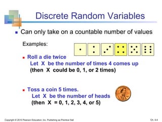
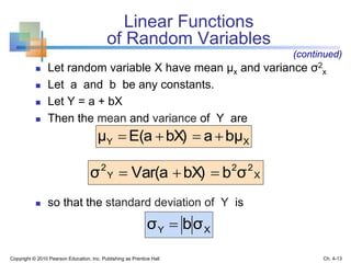
![Functions of Random Variables
If P(x) is the probability function of a discrete
random variable X , and g(X) is some function of
X , then the expected value of function g is
x
g(x)P(x)E[g(X)]
Copyright © 2010 Pearson Education, Inc. Publishing as Prentice Hall Ch. 4-11](https://image.slidesharecdn.com/chap04discreterandomvariablesandprobabilitydistribution-191217014930/85/Chap04-discrete-random-variables-and-probability-distribution-11-320.jpg)
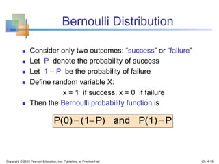
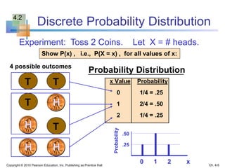
![Bernoulli Distribution
Mean and Variance
The mean is µ = P
The variance is σ2 = P(1 – P)
P(1)PP)(0)(1P(x)xE(X)μ
X
P)P(1PP)(1P)(1P)(0
P(x)μ)(x]μ)E[(Xσ
22
X
222
Copyright © 2010 Pearson Education, Inc. Publishing as Prentice Hall Ch. 4-17](https://image.slidesharecdn.com/chap04discreterandomvariablesandprobabilitydistribution-191217014930/85/Chap04-discrete-random-variables-and-probability-distribution-17-320.jpg)
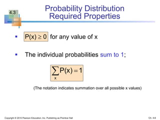
![Poisson Distribution
Characteristics
Mean
Variance and Standard Deviation
λE(X)μ
λ]μ)E[(Xσ 22
λσ
where = expected number of successes per unit
Copyright © 2010 Pearson Education, Inc. Publishing as Prentice Hall Ch. 4-34](https://image.slidesharecdn.com/chap04discreterandomvariablesandprobabilitydistribution-191217014930/85/Chap04-discrete-random-variables-and-probability-distribution-34-320.jpg)
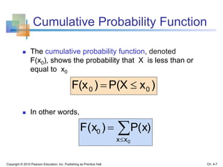
![Conditional Mean and Variance
Ch. 4-41Copyright © 2010 Pearson Education, Inc. Publishing as Prentice Hall
The conditional mean is
The conditional variance is
x)|P(yx)|(yX]|E[Yμ
Y
X|Y
Y
2
X|Y
2
X|Y
2
X|Y x)|x]P(y|)μ[(yX]|)μE[(Yσ](https://image.slidesharecdn.com/chap04discreterandomvariablesandprobabilitydistribution-191217014930/85/Chap04-discrete-random-variables-and-probability-distribution-41-320.jpg)
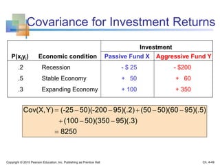
![Covariance
Let X and Y be discrete random variables with means
μX and μY
The expected value of (X - μX)(Y - μY) is called the
covariance between X and Y
For discrete random variables
An equivalent expression is
x y
yxYX y))P(x,μ)(yμ(x)]μ)(YμE[(XY)Cov(X,
x y
yxyx μμy)xyP(x,μμE(XY)Y)Cov(X,
Copyright © 2010 Pearson Education, Inc. Publishing as Prentice Hall Ch. 4-42](https://image.slidesharecdn.com/chap04discreterandomvariablesandprobabilitydistribution-191217014930/85/Chap04-discrete-random-variables-and-probability-distribution-42-320.jpg)
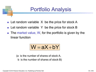
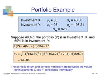
![Portfolio Analysis
The mean value for W is
The variance for W is
or using the correlation formula
(continued)
YX
W
bμaμ
bY]E[aXE[W]μ
Y)2abCov(X,σbσaσ 2
Y
22
X
22
W
YX
2
Y
22
X
22
W σY)σ2abCorr(X,σbσaσ
Copyright © 2010 Pearson Education, Inc. Publishing as Prentice Hall Ch. 4-46](https://image.slidesharecdn.com/chap04discreterandomvariablesandprobabilitydistribution-191217014930/85/Chap04-discrete-random-variables-and-probability-distribution-46-320.jpg)
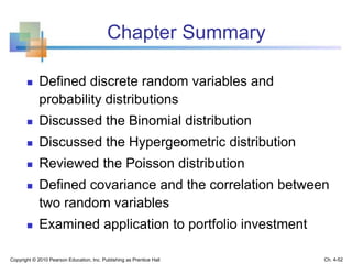

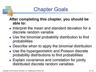
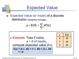
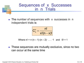
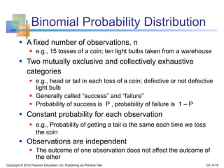
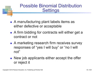
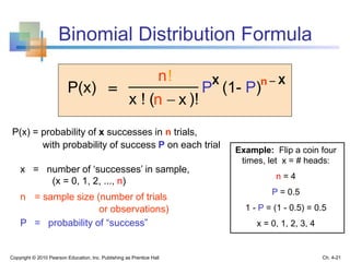
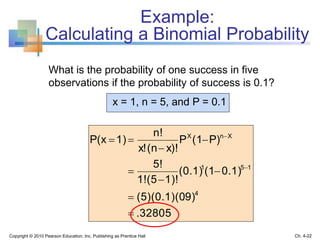
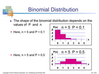
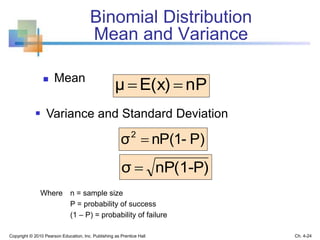
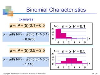
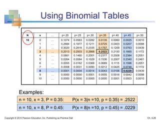
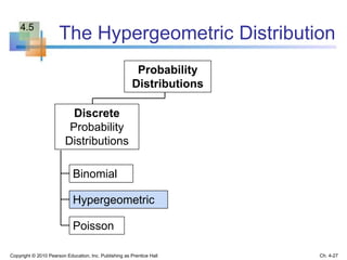
This document provides an overview of key concepts in chapter 4 of the textbook "Statistics for Business and Economics". The chapter goals are to understand mean, standard deviation, and probability distributions for discrete random variables, including the binomial, hypergeometric, and Poisson distributions. It introduces discrete random variables and probability distributions, and defines important properties like expected value, variance, and cumulative probability functions. It also covers the Bernoulli distribution as well as the characteristics and applications of the binomial distribution.