Downloaded 174 times

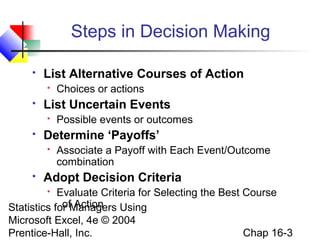


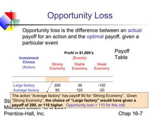

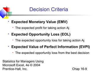


This document provides an overview of key concepts in decision making covered in Chapter 16 of the textbook "Statistics for Managers Using Microsoft Excel". It begins by listing the chapter goals, which include describing decision making processes, constructing decision tables, applying expected value criteria, and accounting for risk attitudes. It then outlines the typical steps in decision making, such as listing alternatives and possible outcomes. Key decision making criteria are defined, like expected monetary value, expected opportunity loss, and value of perfect information. Examples are provided to demonstrate how to apply these concepts to make optimal decisions under uncertainty.


