Downloaded 304 times


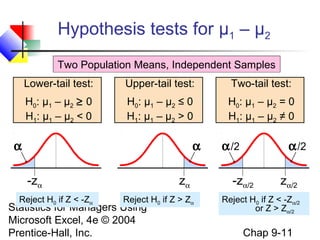


This chapter discusses two-sample tests, including tests for the difference between two independent population means, the difference between two related (paired) sample means, the difference between two population proportions, and the difference between two variances. It provides the formulas and procedures for conducting Z tests, t tests, and F tests for these comparisons in situations where the population standard deviations are both known and unknown. The goal is to test hypotheses about differences between parameters of two populations or to construct confidence intervals for these differences.