Downloaded 123 times

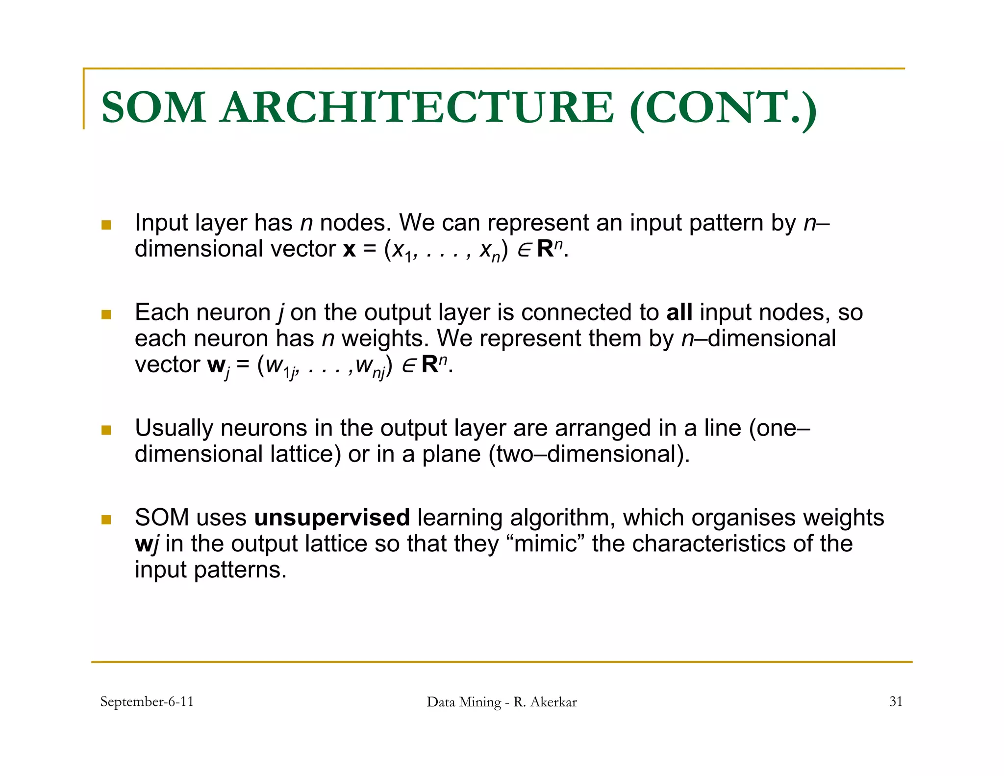
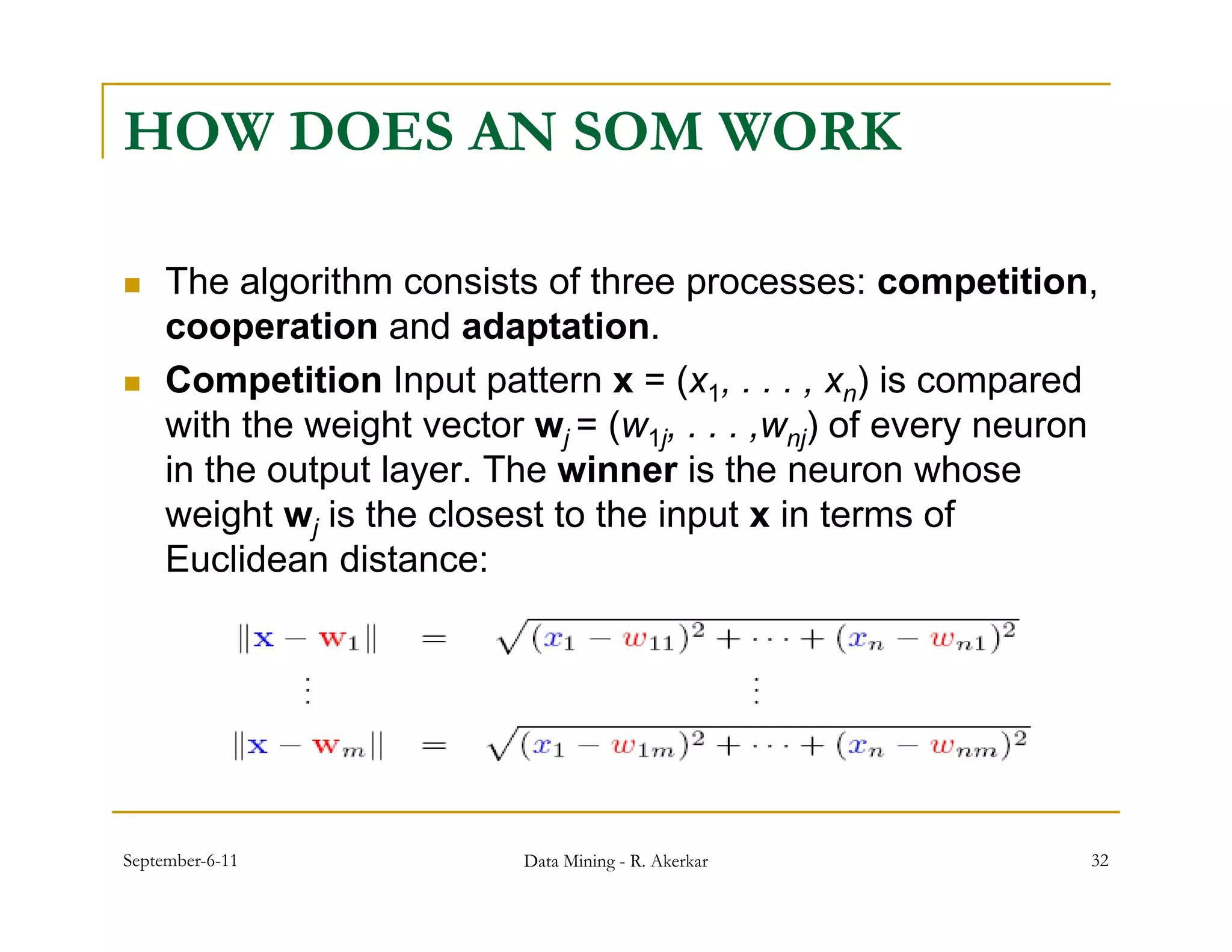
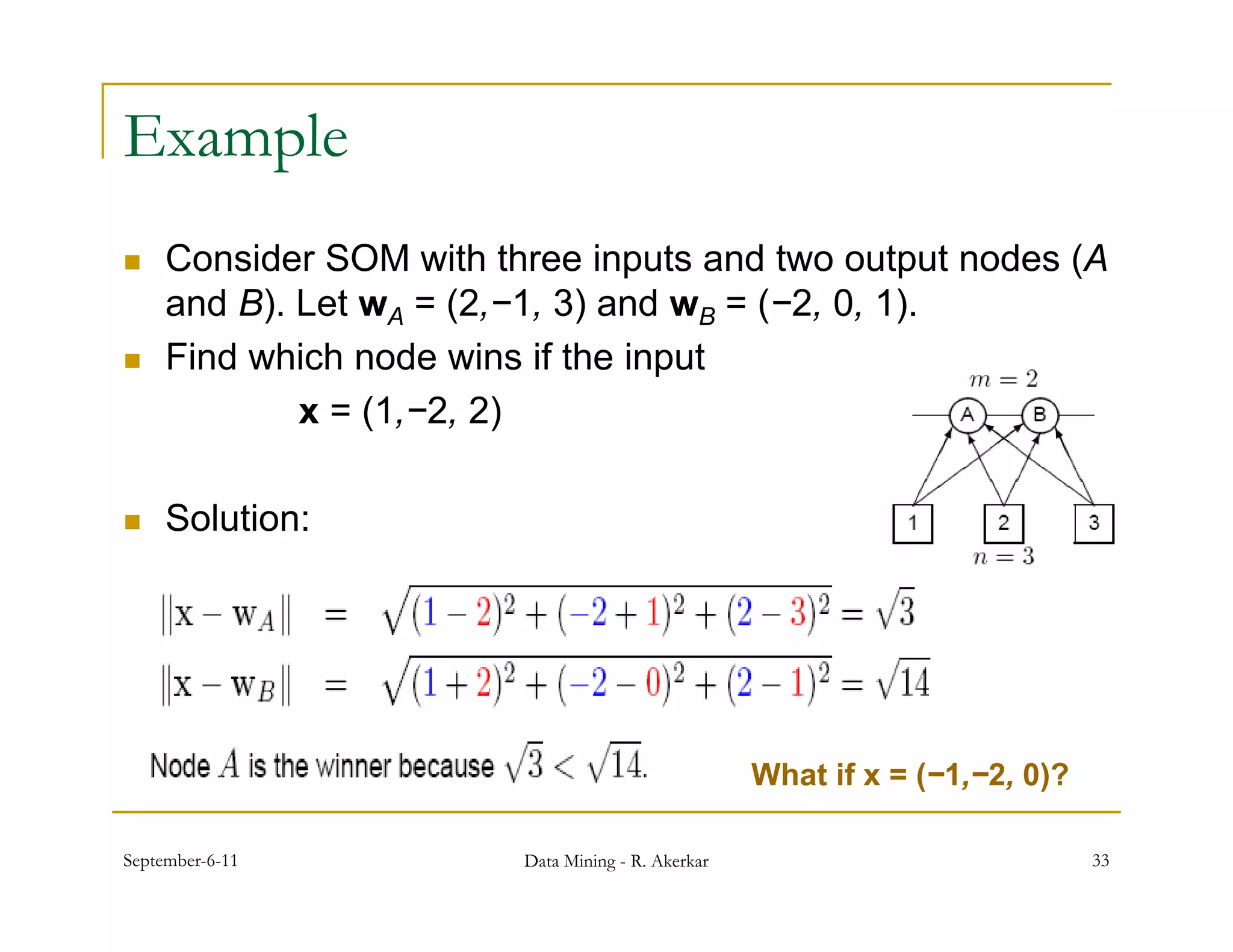
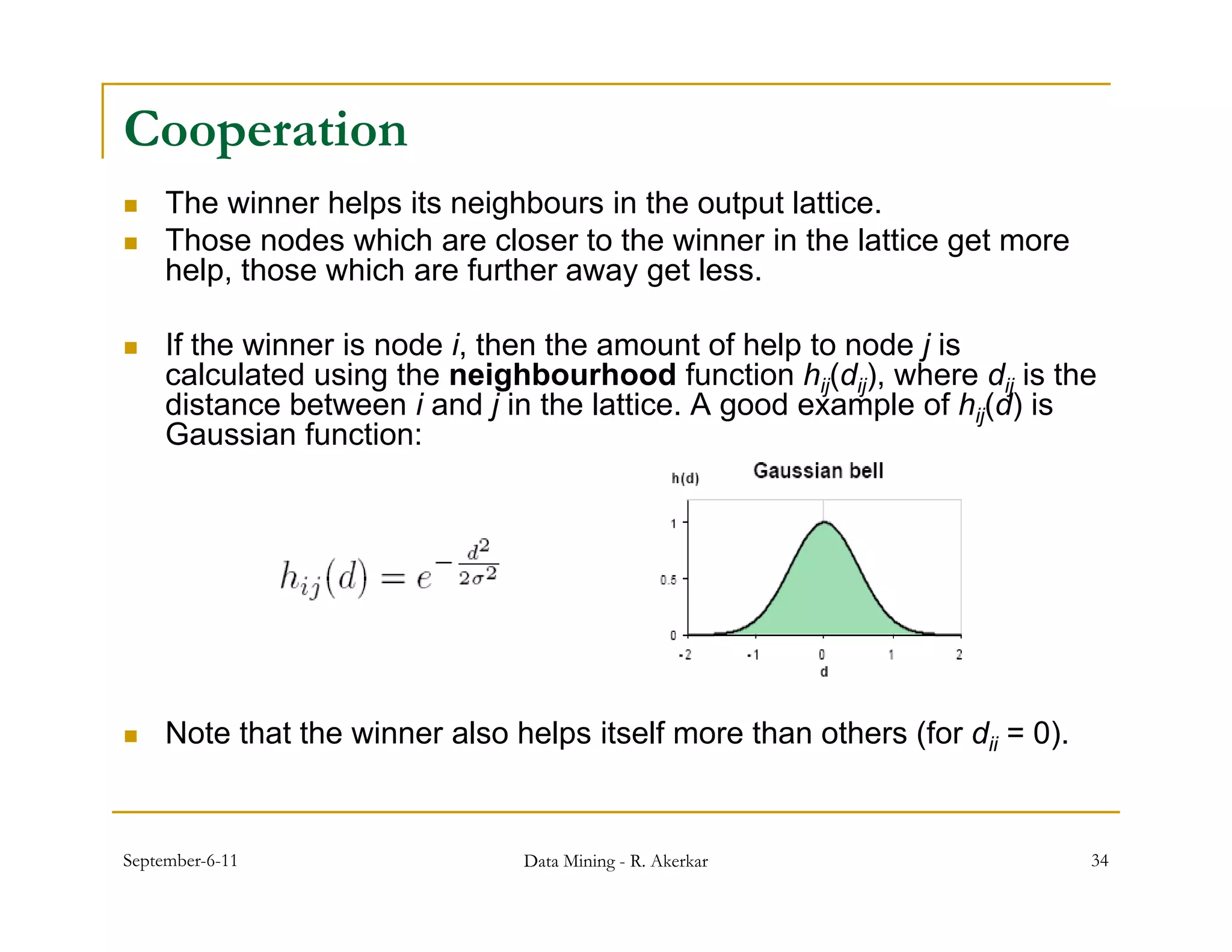
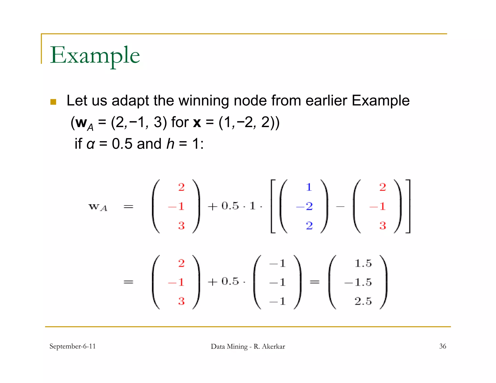
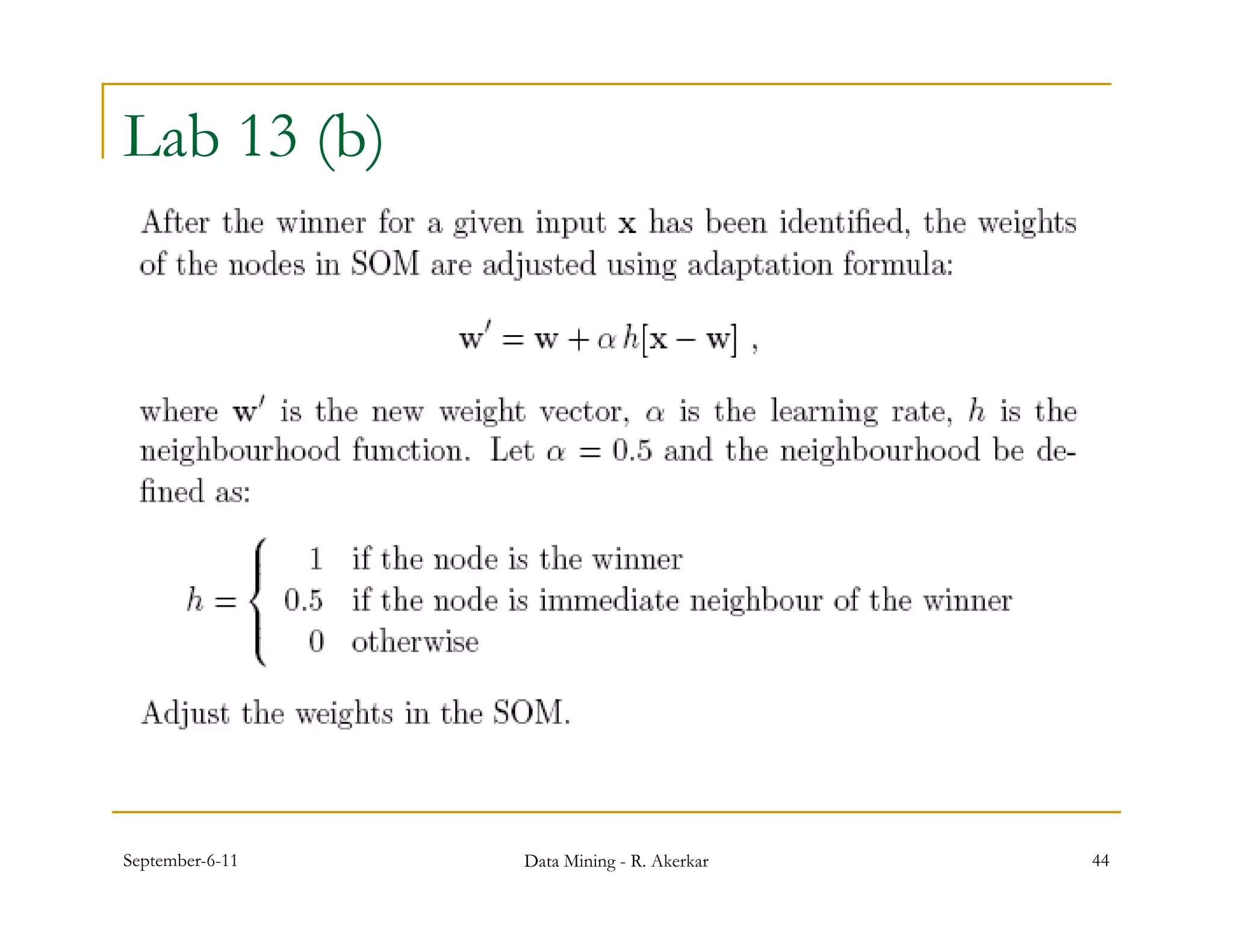
![Adaptation
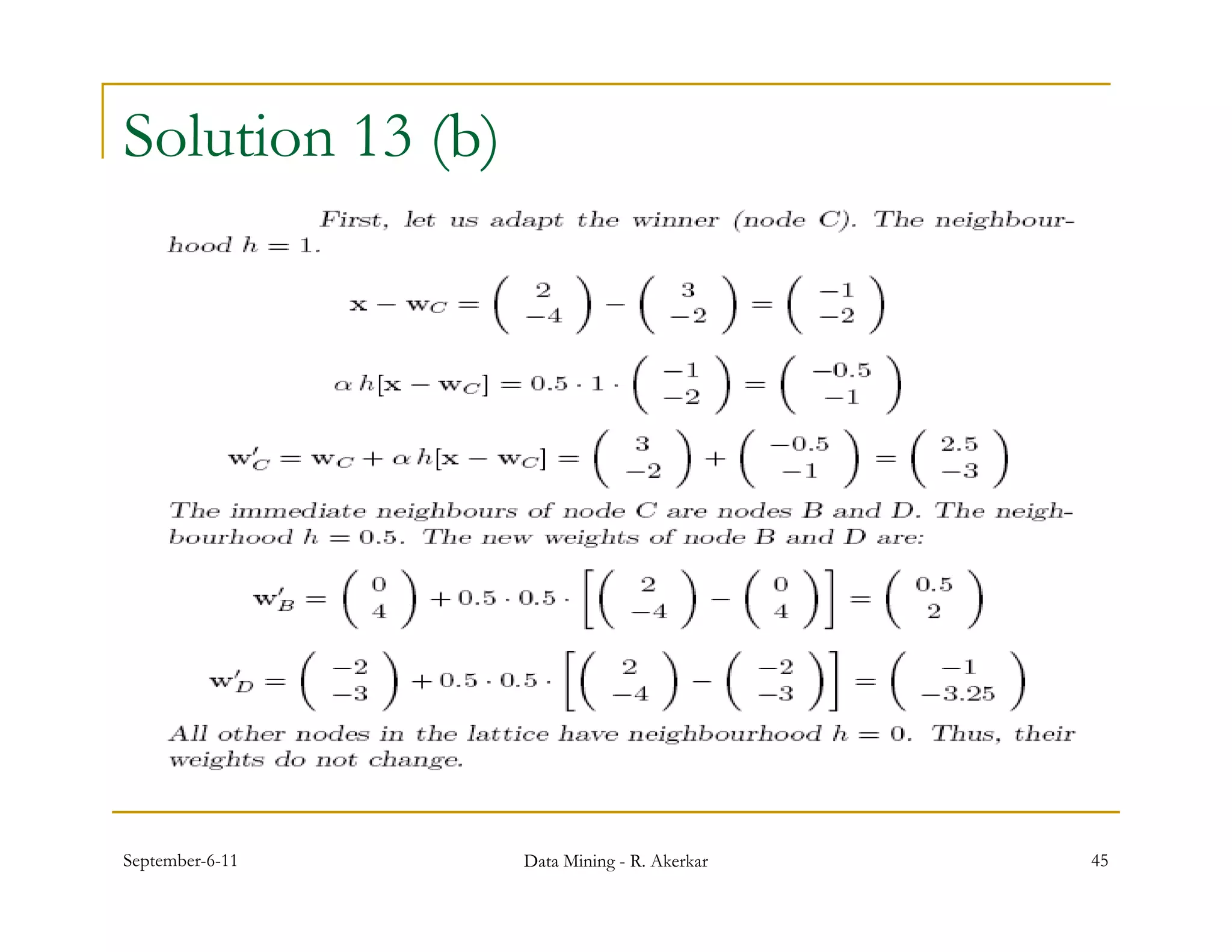
After the input x has been presented to SOM, the weights wj of
the nodes are adjusted so that they become “closer” to the input.
The exact formula for adaptation of weights is:
w’j = wj + αhij [x − wj ] ,
where α is the learning rate coefficient.
One can see that the amount of change depends on the
neighbourhood hij of the winner. So, the winner helps itself and
its neighbours to adapt.
Finally, the neighbourhood hij is also a function of time, such that
the neighbourhood shrinks with time (e.g. σ decreases with t).
September-6-11 Data Mining - R. Akerkar 35](https://image.slidesharecdn.com/neuralnets-110906041700-phpapp02/75/Neural-Networks-35-2048.jpg)

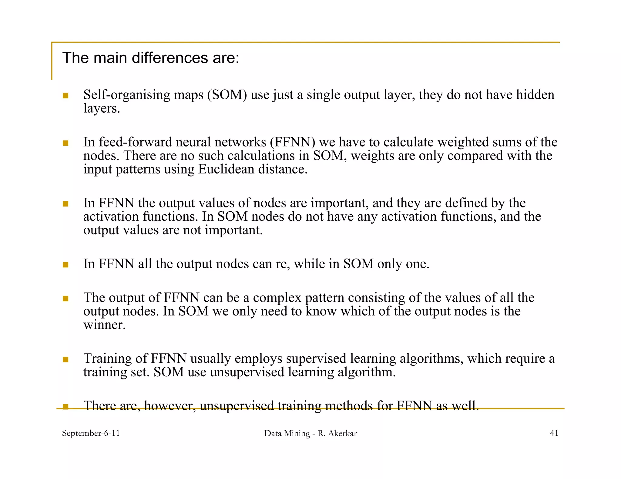
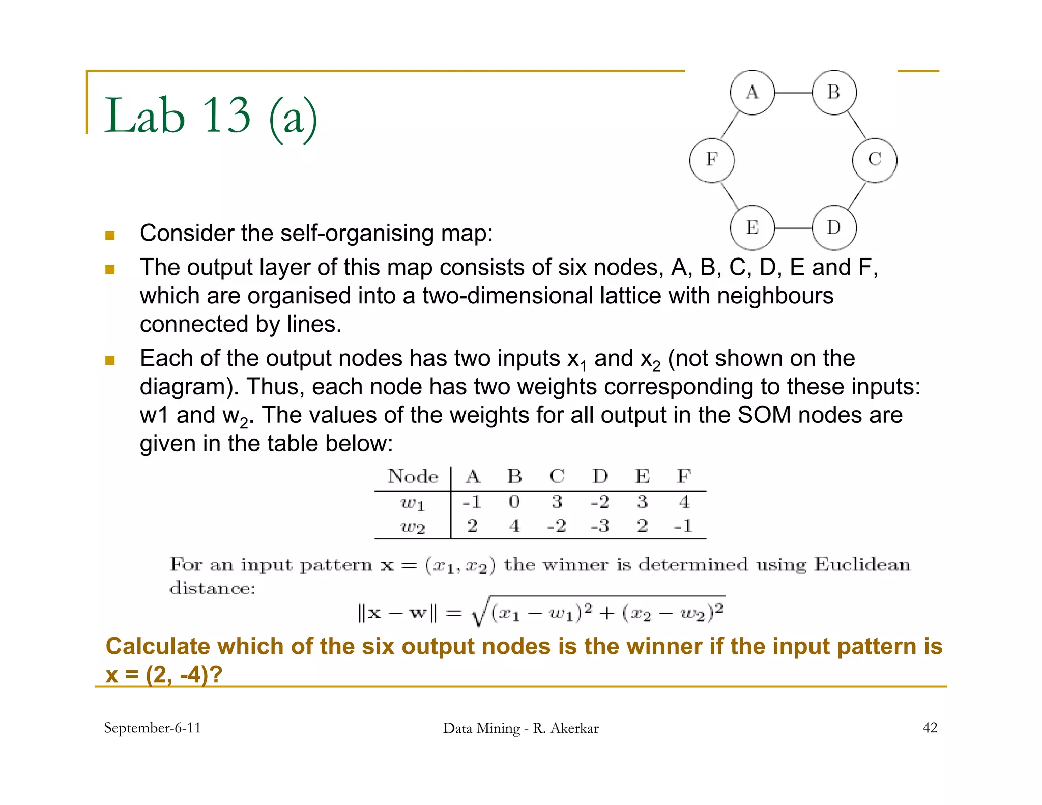
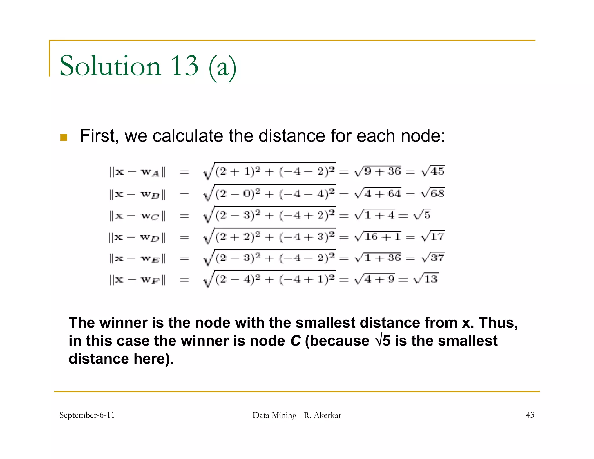

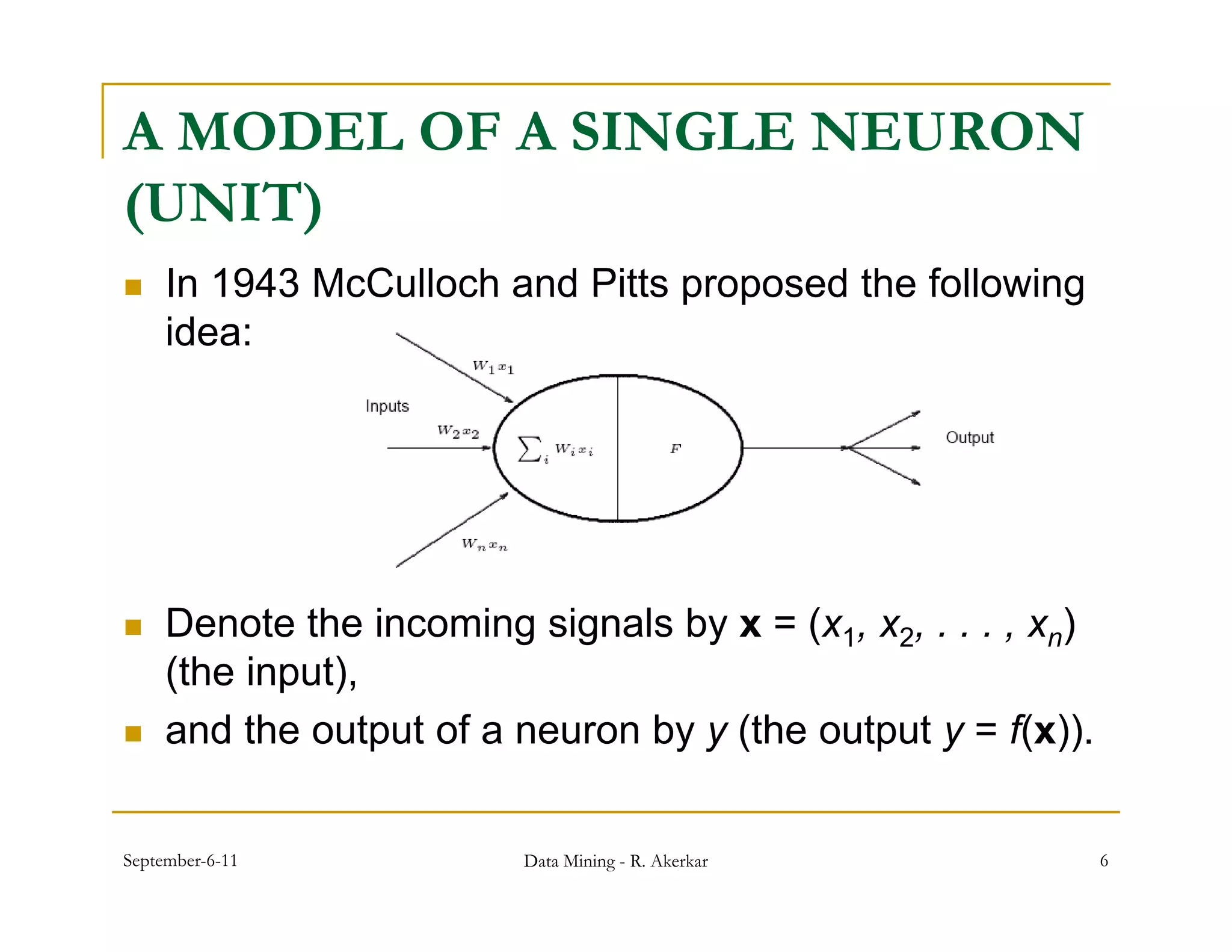
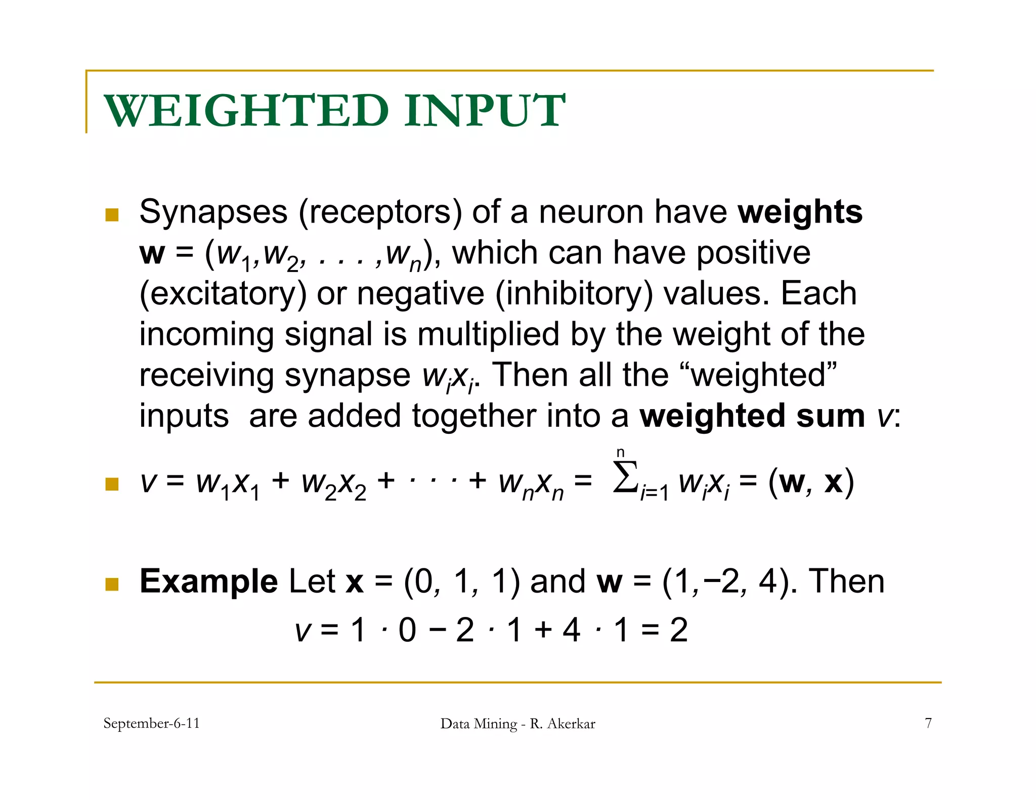
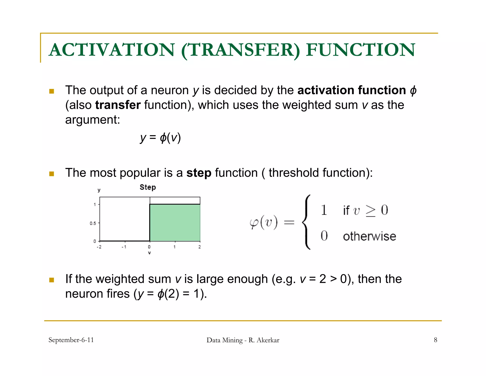
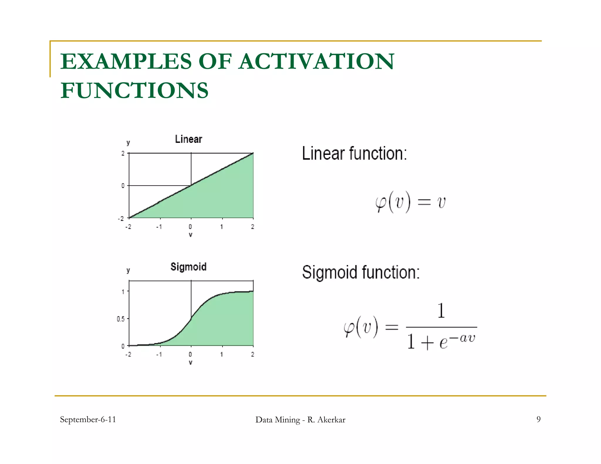
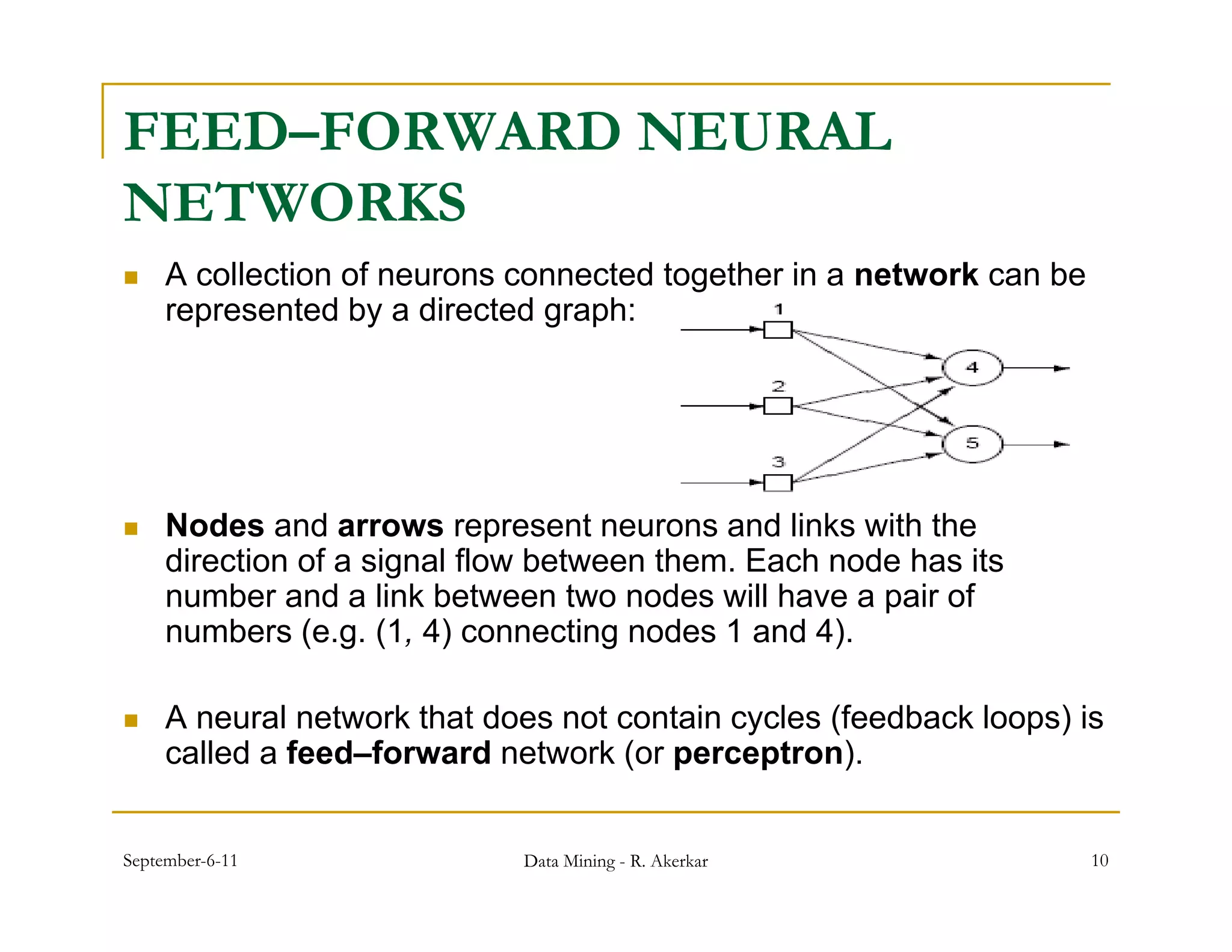
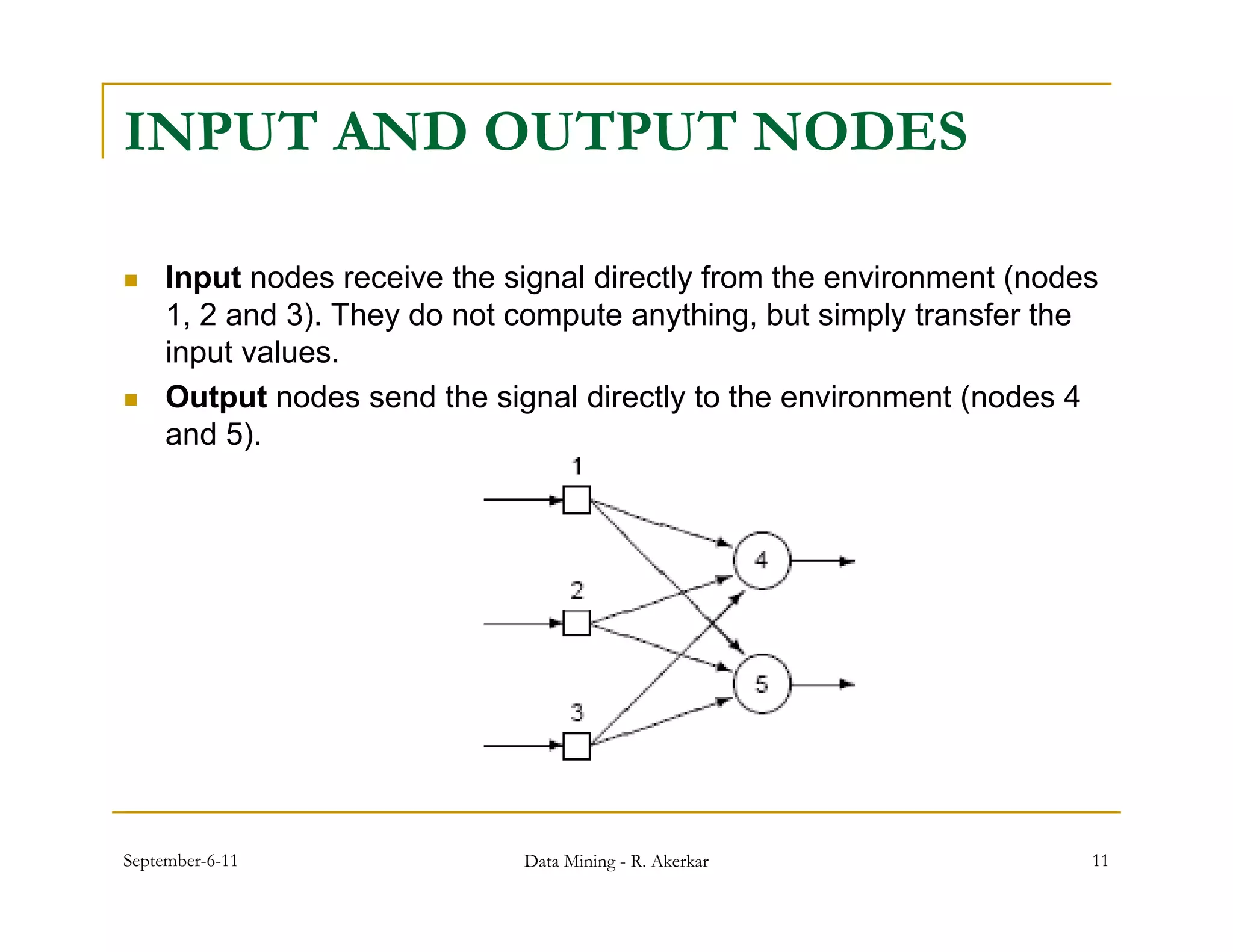
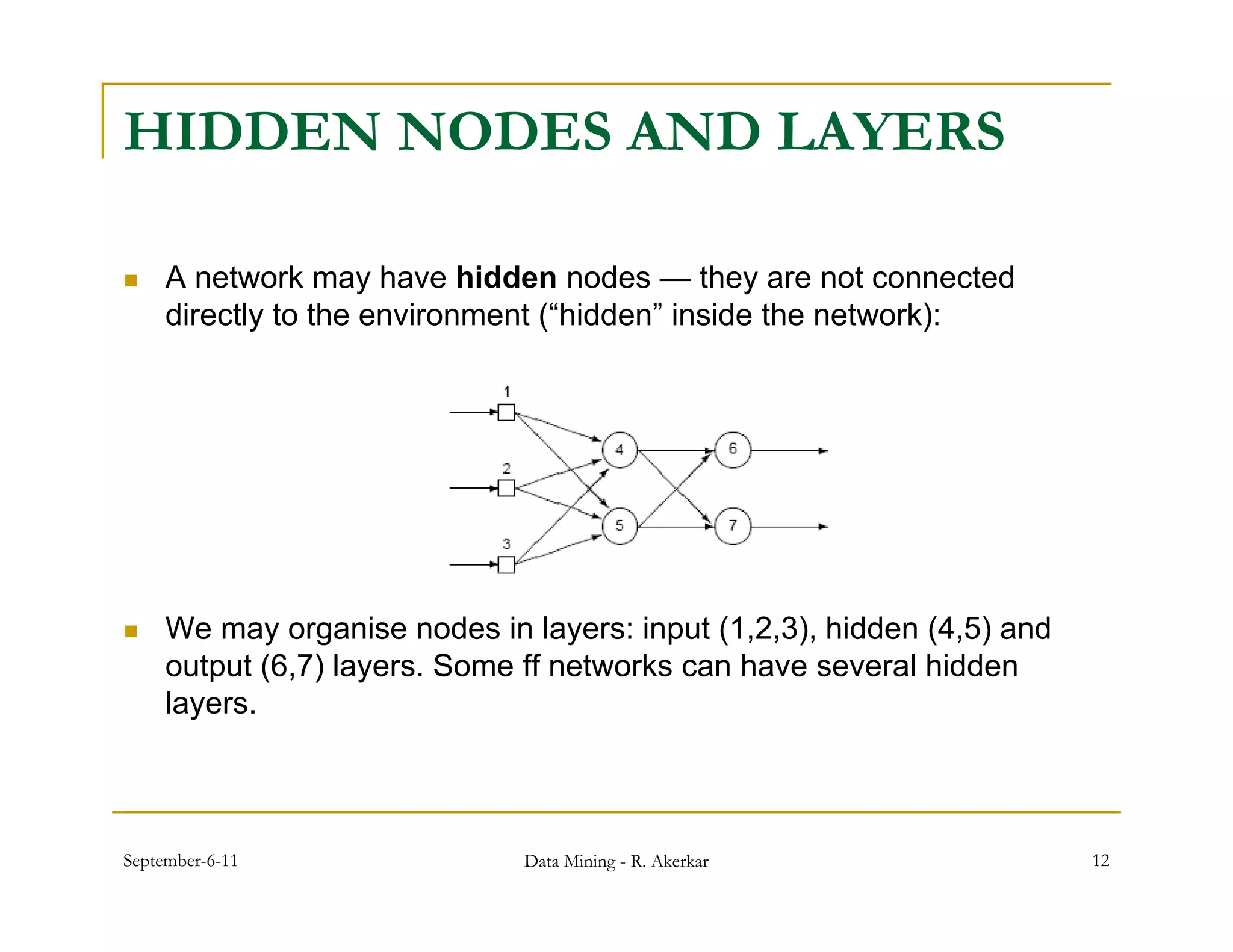
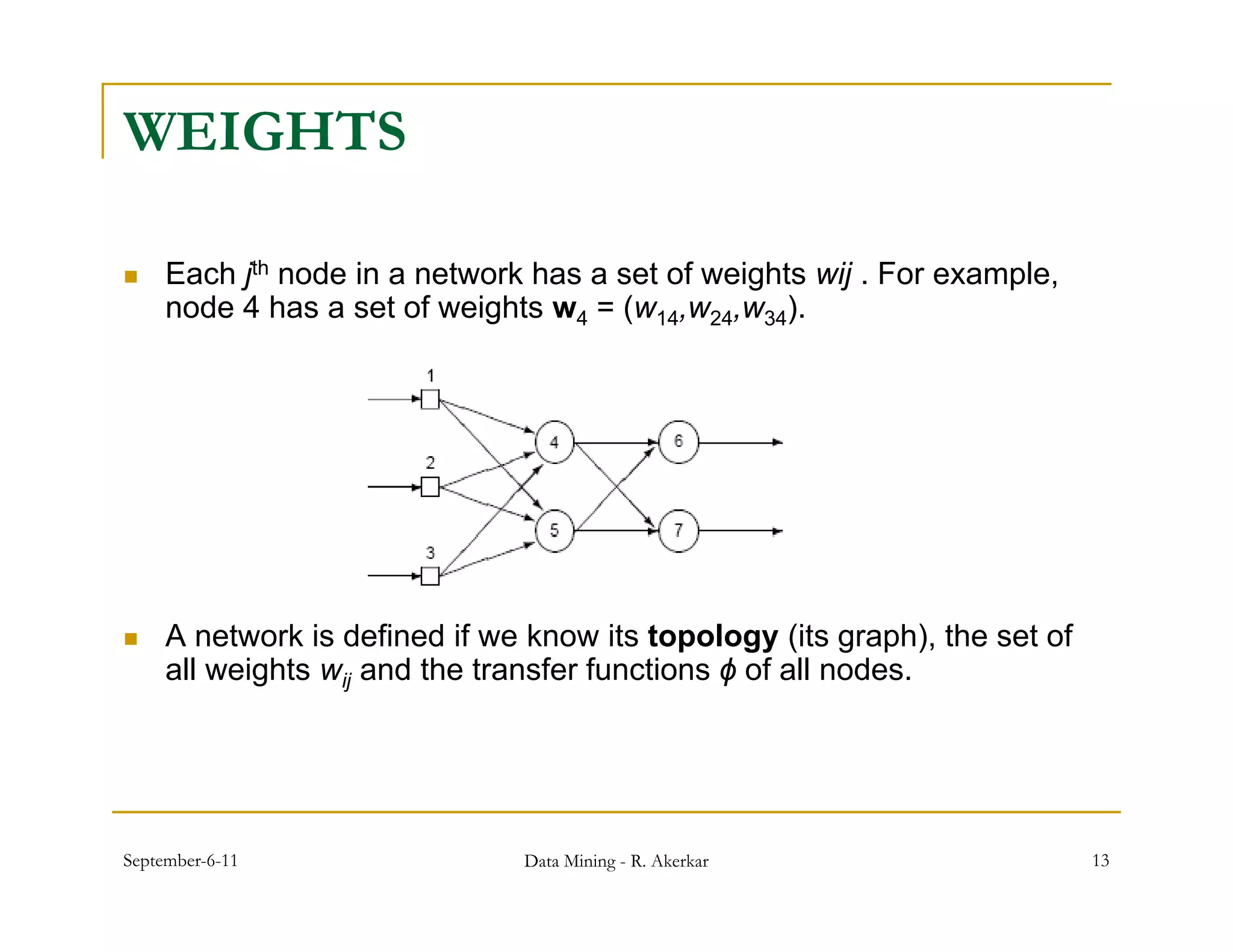
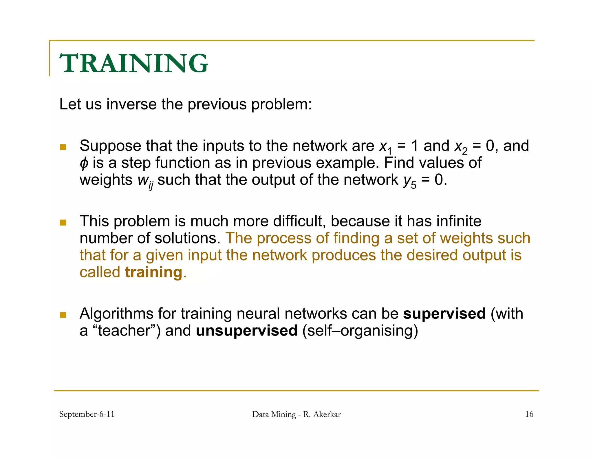
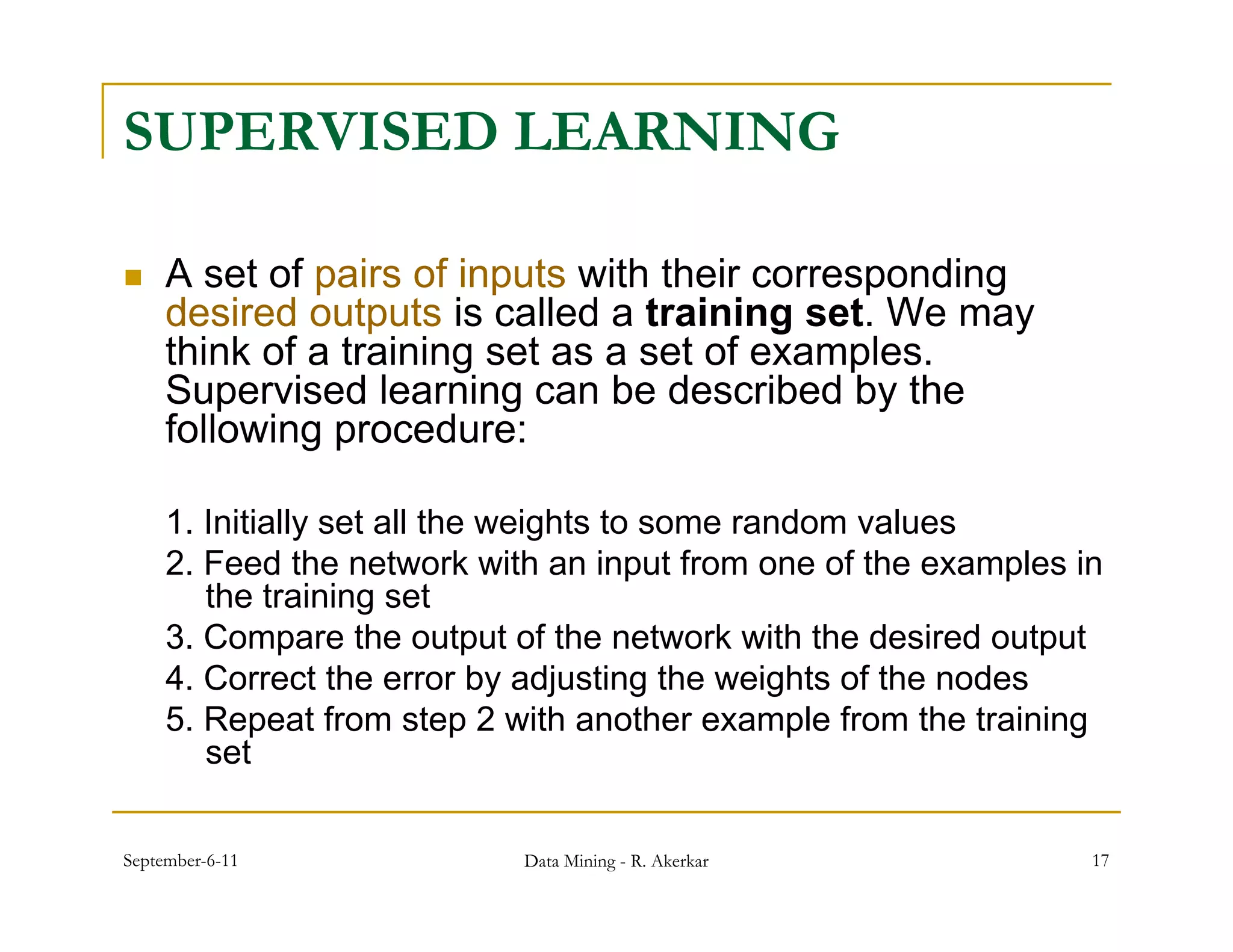
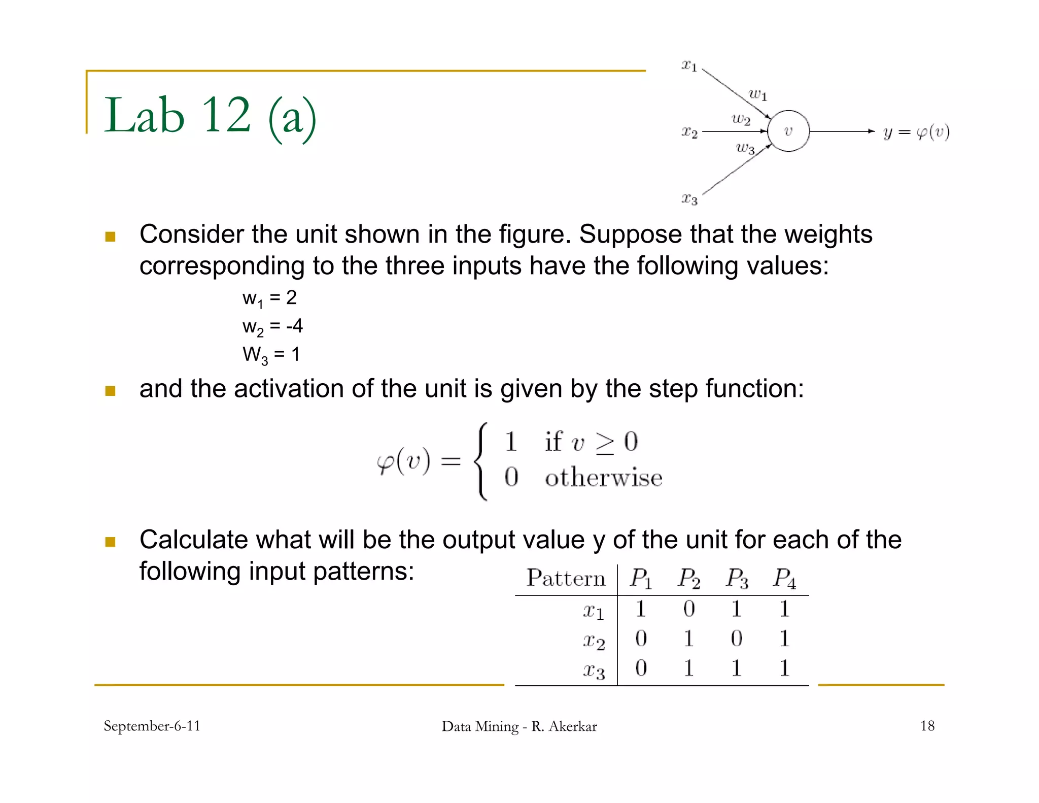
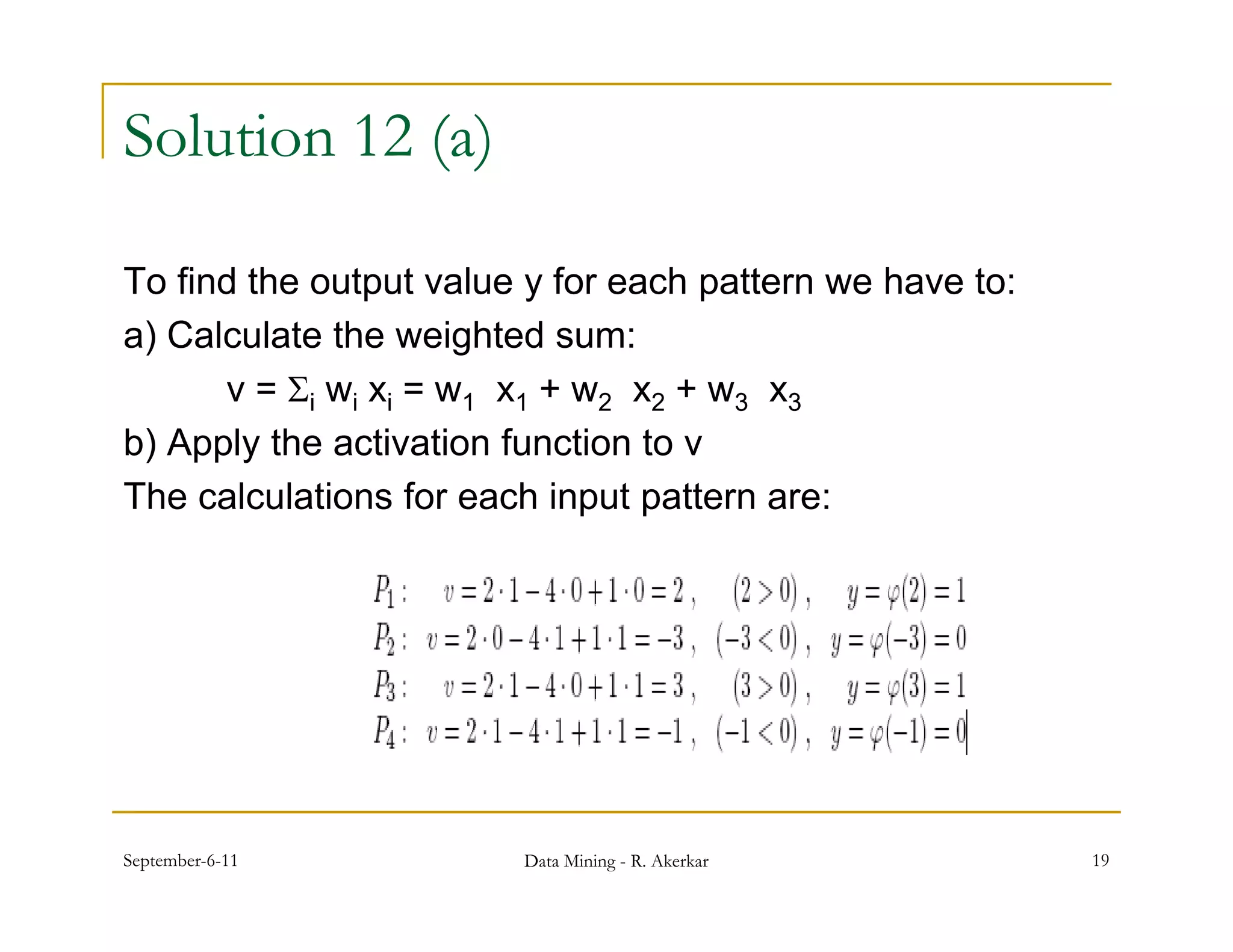
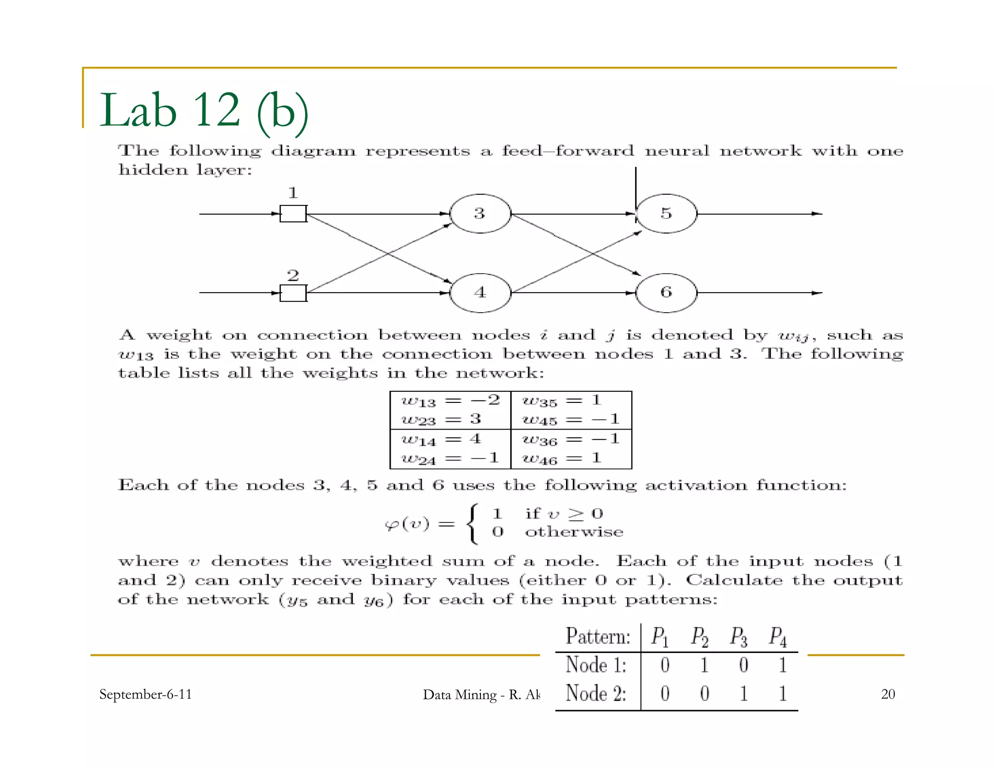
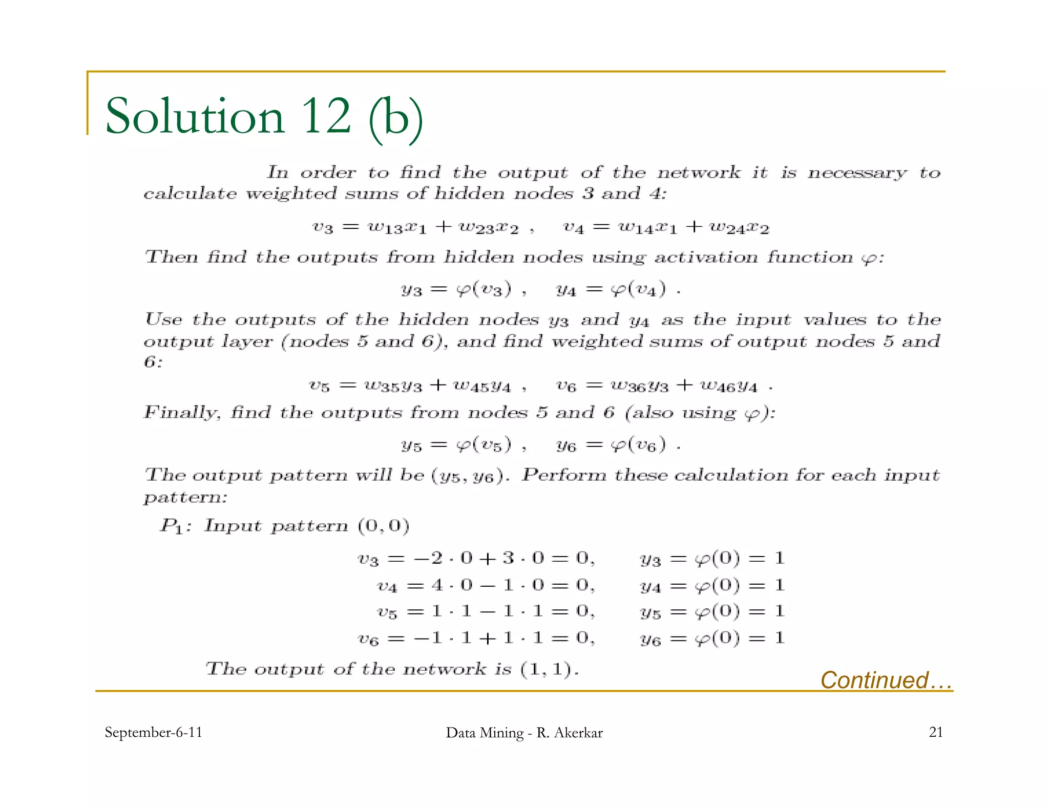
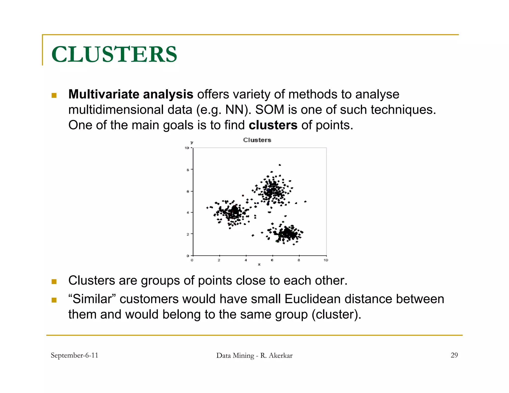
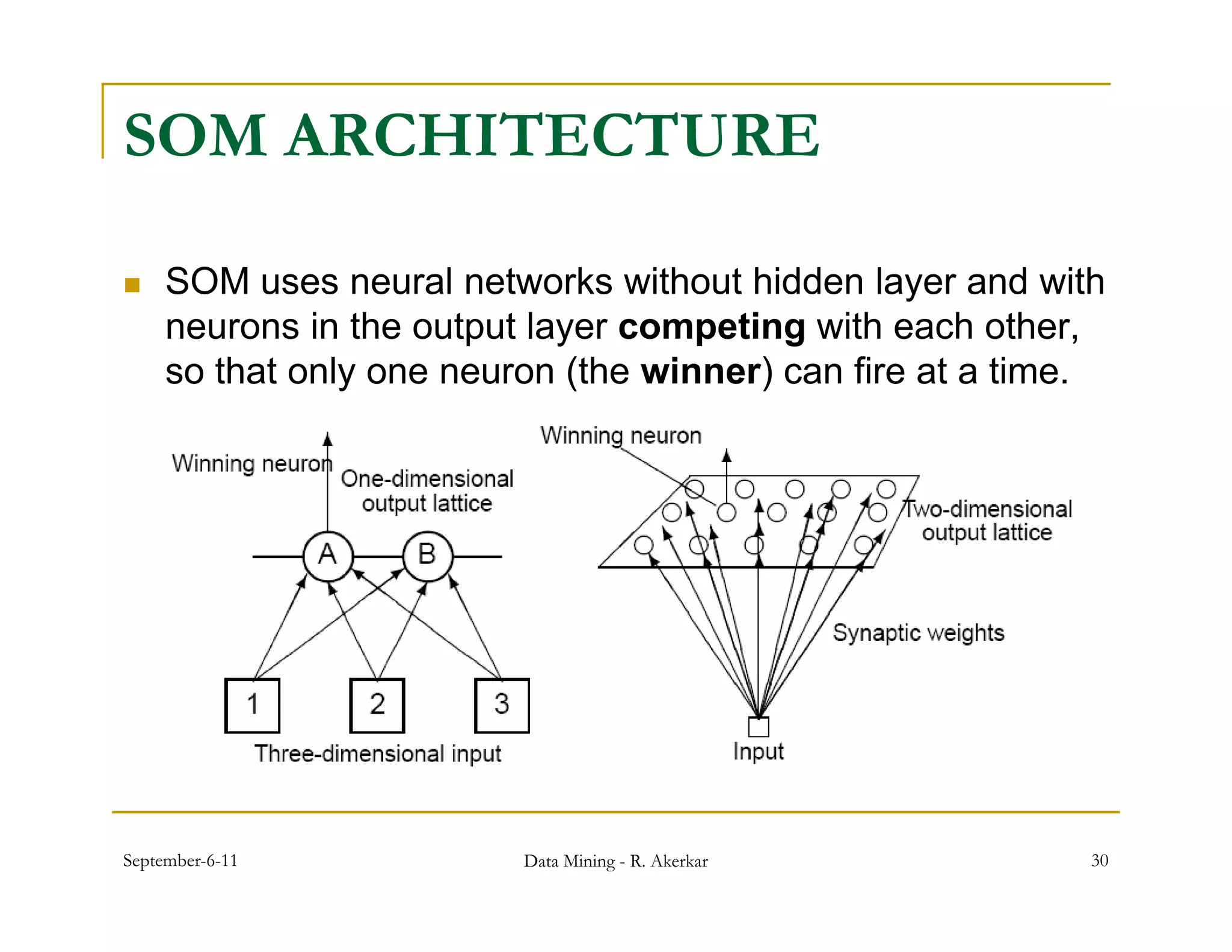
1. Feed-forward neural networks are composed of nodes connected in a directed graph without feedback loops. Information flows from input to output nodes through one or more hidden layers. 2. Each node receives weighted input signals, calculates a weighted sum, and applies an activation function to determine its output. During training, weights are adjusted to minimize error between network outputs and desired targets. 3. Self-organizing maps are neural networks that use unsupervised learning to produce a low-dimensional representation of input patterns. They cluster multidimensional data onto a two-dimensional map based on topological similarity.