Download as PDF, PPTX


![ASU-CSC445: Neural Networks Prof. Dr. Mostafa Gadal-Haqq
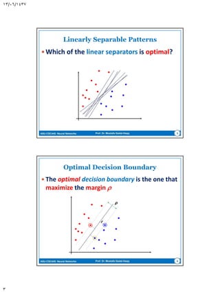
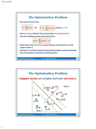
The Optimization Problem
Introduce Lagrange multipliers ,
That is, the Lagrange function:
Is to be minimized with respect to w and b, i.e,
𝜕𝑱(𝒘,𝒃,)
𝜕𝒘
= 𝟎 ; and
𝜕𝑱(𝒘,𝒃, )
𝜕𝒃
= 𝟎
)1][(||||
2
1
),,(
1
2
bxwdwbwJ i
T
i
N
i
i
11](https://image.slidesharecdn.com/xfr2zudmqrylir8lbcjv-signature-7f7e9932c1ac6134e9030bbdd4cfa1c5606f58d572ef5d7da58609957cc1fc67-poli-160617131027/85/Neural-Networks-Support-Vector-machines-11-320.jpg)


![ASU-CSC445: Neural Networks Prof. Dr. Mostafa Gadal-Haqq
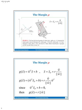
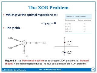
The XOR Problem
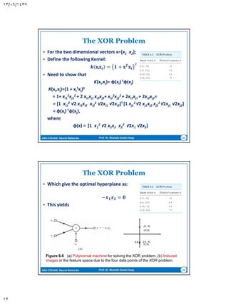
For the two dimensional vectors x=[x1 x2];
Define the following Kernel:
𝒌 x,x𝒊 = 𝟏 + x 𝑻
x𝒊
2
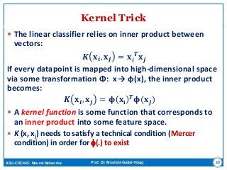
Need to show that
K(xi,xj)= φ(xi)Tφ(xj)
K(xi,xj)=(1 + xi
Txj)2
= 1+ xi1
2xj1
2 + 2 xi1xj1 xi2xj2+ xi2
2xj2
2 + 2xi1xj1 + 2xi2xj2=
= [1 xi1
2 √2 xi1xi2 xi2
2 √2xi1 √2xi2]T [1 xj1
2 √2 xj1xj2 xj2
2 √2xj1 √2xj2]
= φ(xi)Tφ(xj),
where
φ(x) = [1 x1
2 √2 x1x2 x2
2 √2x1 √2x2]
23](https://image.slidesharecdn.com/xfr2zudmqrylir8lbcjv-signature-7f7e9932c1ac6134e9030bbdd4cfa1c5606f58d572ef5d7da58609957cc1fc67-poli-160617131027/85/Neural-Networks-Support-Vector-machines-23-320.jpg)


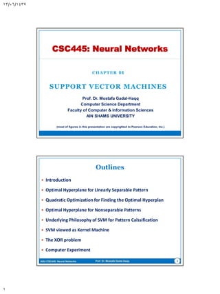
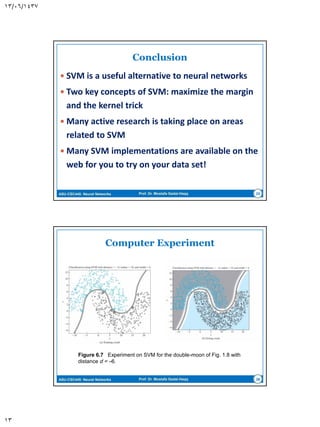
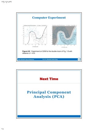
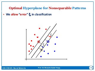
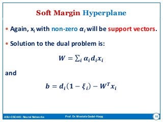
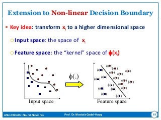
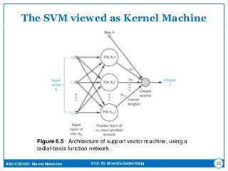
This document discusses support vector machines (SVMs) for pattern classification. It begins with an introduction to SVMs, noting that they construct a hyperplane to maximize the margin of separation between positive and negative examples. It then covers finding the optimal hyperplane for linearly separable and nonseparable patterns, including allowing some errors in classification. The document discusses solving the optimization problem using quadratic programming and Lagrange multipliers. It also introduces the kernel trick for applying SVMs to non-linear decision boundaries using a kernel function to map data to a higher-dimensional feature space. Examples are provided of applying SVMs to the XOR problem and computer experiments classifying a double moon dataset.