Download as PDF, PPTX
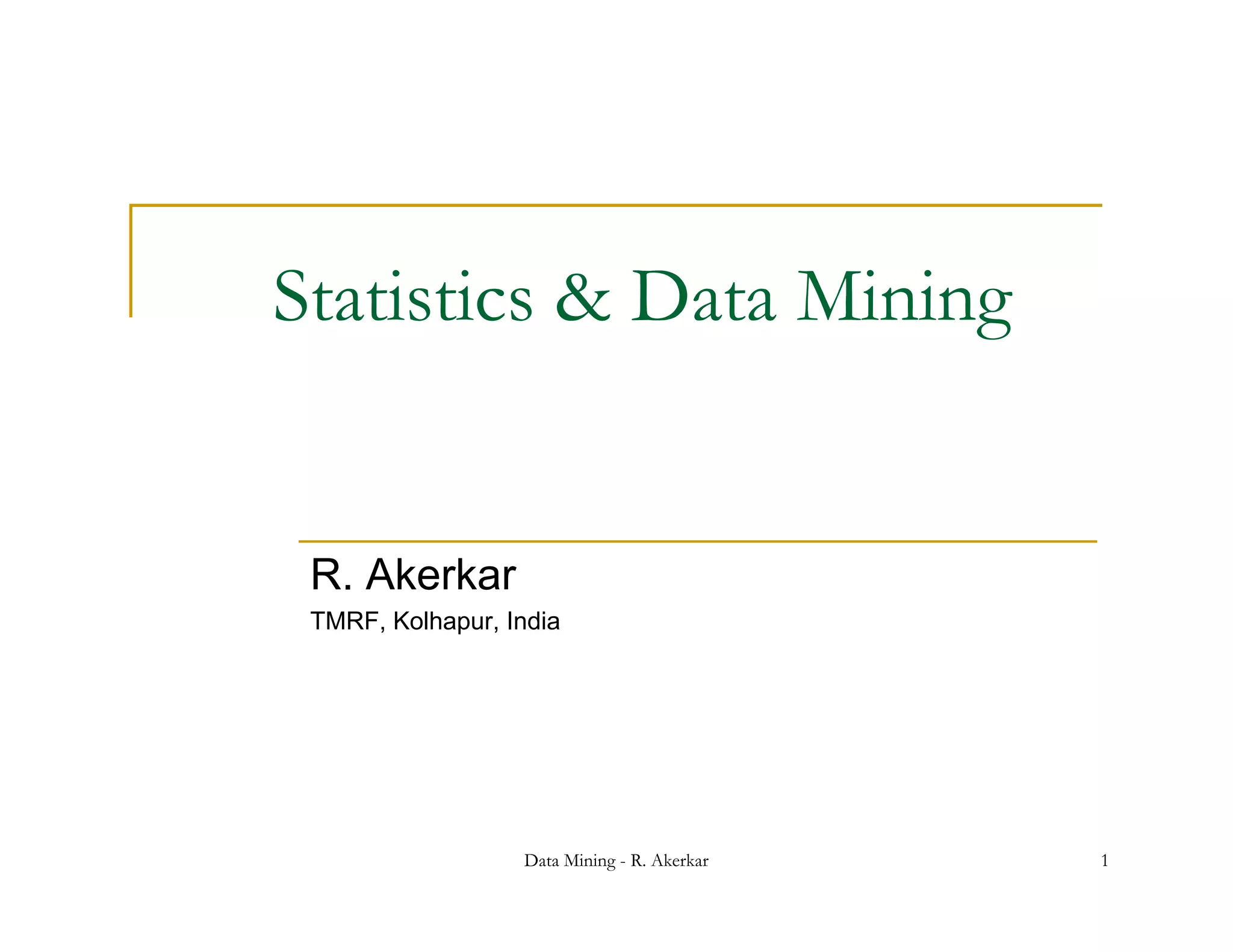
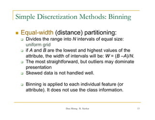
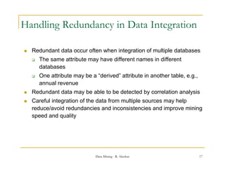
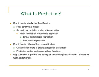
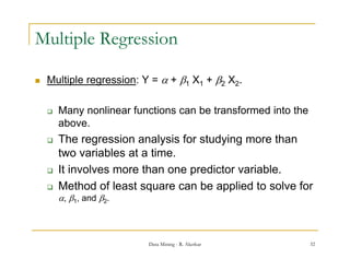
![Data Transformation: Normalization
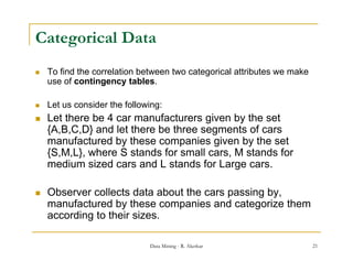
min-max normalization (This type of normalization transforms the data into a
desired range, usually [0,1]. )
v minA
v' (new _ maxA new _ minA) new _ minA
maxA minA
where, [minA, maxA] is the initial range and [new_minA, new_maxA] is the
,[ , ] g [ , ]
new range.
e.g.: If v = 73600 in [12000, 98000] Then v’ = 0.716 in the range [0, 1].
Here value for “income” is transformed to 0.716
It preserves the relationship among th original d t values.
th l ti hi the i i l data l
Data Mining - R. Akerkar 24](https://image.slidesharecdn.com/statdm-110906051117-phpapp01/85/Statistics-and-Data-Mining-24-320.jpg)
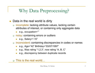
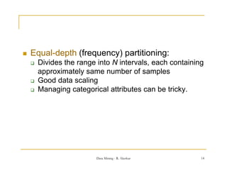
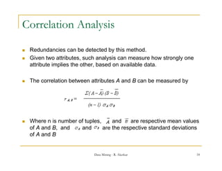
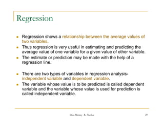
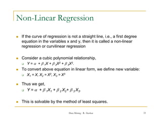
![Normalisation by Decimal Scaling
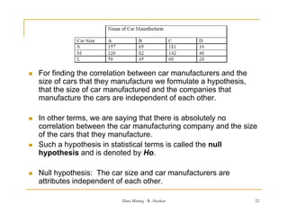
This type of scaling transforms the data into a range between [-
1,1]. The transformation formula is
v
v' j
10
Where j is the smallest integer such that Max(| v' |)<1
e.g.: Suppose recorded value of A is in initial range [-991, 99], k is
3, and v = -991 becomes v' = -0.991.
The
Th mean absolute value of A is 991.
b l t l f i 991
To normalise, we divide each value by 1000 (i.e. j = 3) so -991
normalises -0.991
Data Mining - R. Akerkar 26](https://image.slidesharecdn.com/statdm-110906051117-phpapp01/85/Statistics-and-Data-Mining-26-320.jpg)
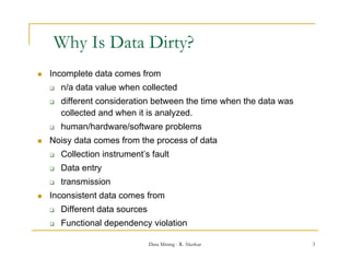
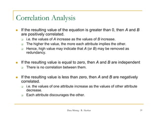
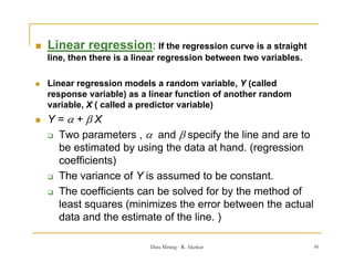
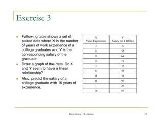
![Exercise 2
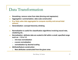
Using the data for Age in previous Question, answer the following:
a) Use min-max normalization to transform the value 35 for age into the
range [0.0; 1.0].
b) Use z-score normalization to transform the value 35 for age, where
the standard deviation of age is 12.94.
c) Use normalization by decimal scaling to transform the value 35 for
age.
d) Comment on which method you would prefer to use for the given
data, giving reasons as to why.
Data Mining - R. Akerkar 27](https://image.slidesharecdn.com/statdm-110906051117-phpapp01/85/Statistics-and-Data-Mining-27-320.jpg)

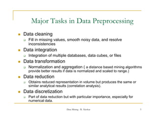
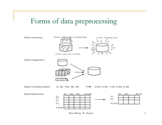
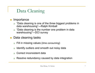
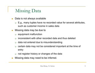
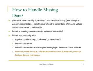
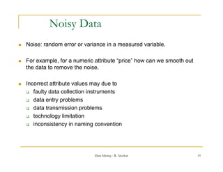
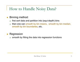
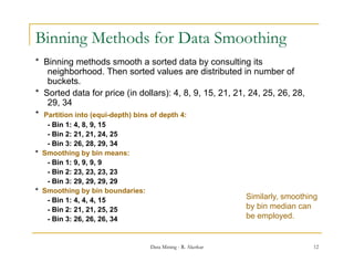
This document discusses data preprocessing techniques for data mining. It explains that real-world data is often dirty, containing issues like missing values, noise, and inconsistencies. Major tasks in data preprocessing include data cleaning, integration, transformation, reduction, and discretization. Data cleaning techniques are especially important and involve filling in missing values, identifying and handling outliers, resolving inconsistencies, and reducing redundancy from data integration. Other techniques discussed include binning data for smoothing noisy values and handling missing data through various imputation methods.