Download as PDF, PPTX
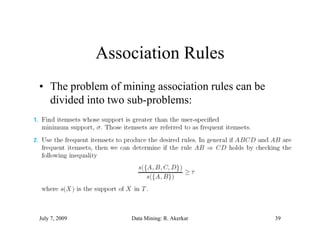
![From [Fayyad, et.al.] Advances in Knowledge Discovery and Data Mining, 1996
[ yy , ] g y g,
July 7, 2009 Data Mining: R. Akerkar 4](https://image.slidesharecdn.com/datamining-111106092900-phpapp01/85/Data-mining-4-320.jpg)
![The S
Th Square-error of th cluster
f the l t
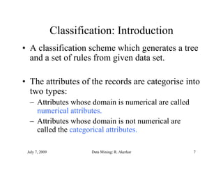
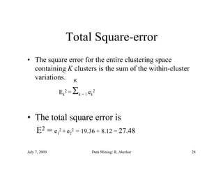
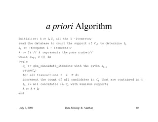
• The square-error for cluster Ck is the sum of squared Euclidean
distances between each sample in Ck and its centroid.
• Thi error is called the within-cluster variation.
This i ll d th ithi l t i ti
ek2 = n k
i=1 (xik – Mk)2
• Within cluster variations, after initial random distribution of
samples, are
• e12 = [(0 – 1.66)2 + (2 – 0.66)2] + [(0 – 1.66)2 + (0 – 0.66)2]
+ [(5 – 1.66)2 + (0 – 0.66)2] = 19.36
• e22 = [(1.5 – 3.25)2 + (0 – 1)2] + [( – 3.25)2 + (2 – 1)2] = 8.12
[( ) ( ) [(5 ) ( )
July 7, 2009 Data Mining: R. Akerkar 27](https://image.slidesharecdn.com/datamining-111106092900-phpapp01/85/Data-mining-27-320.jpg)

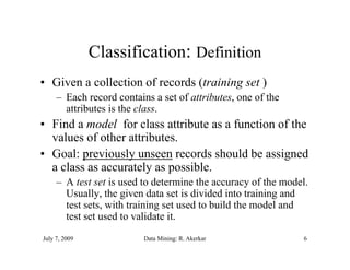
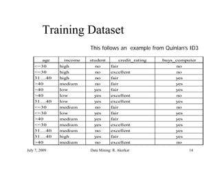
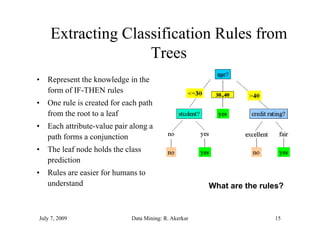
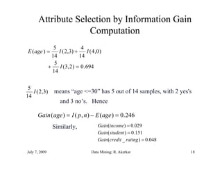
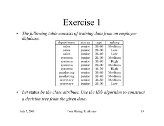
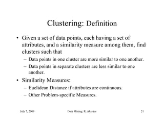
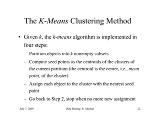
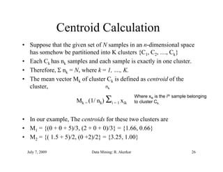
The document discusses data mining and classification techniques. It defines data mining as the extraction of interesting patterns from large amounts of data. Classification involves using attributes of records in a training dataset to predict the class of new, unseen records. Decision trees are a common classification technique that use attributes to recursively split data into subgroups until each subgroup belongs to a single class. The document also discusses clustering, which organizes unlabeled data into groups without predefined classes.