Downloaded 295 times
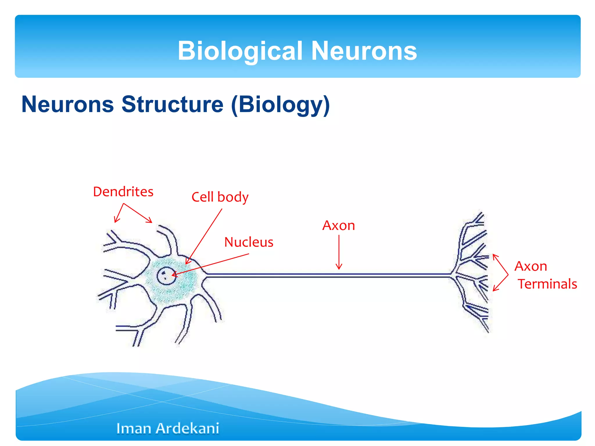
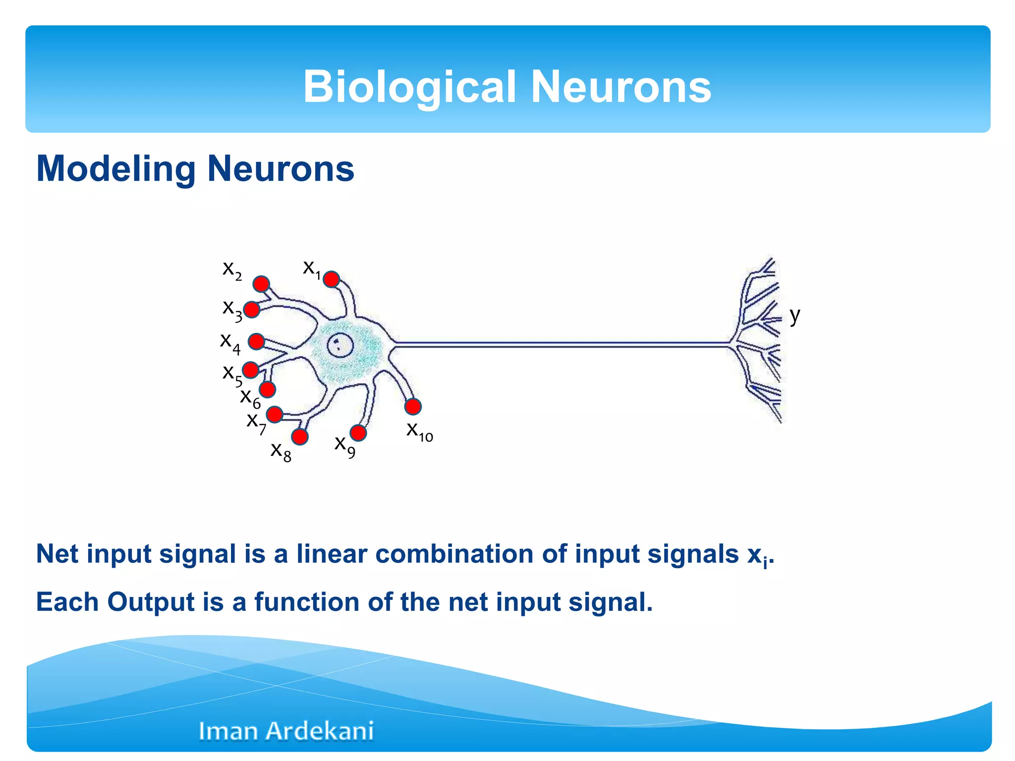
![Net input signal received through synaptic junctions is
net = b + Σwixi = b + WT
X
Weight vector: W =[w1 w2 … wm]T
Input vector: X = [x1 x2 … xm]T
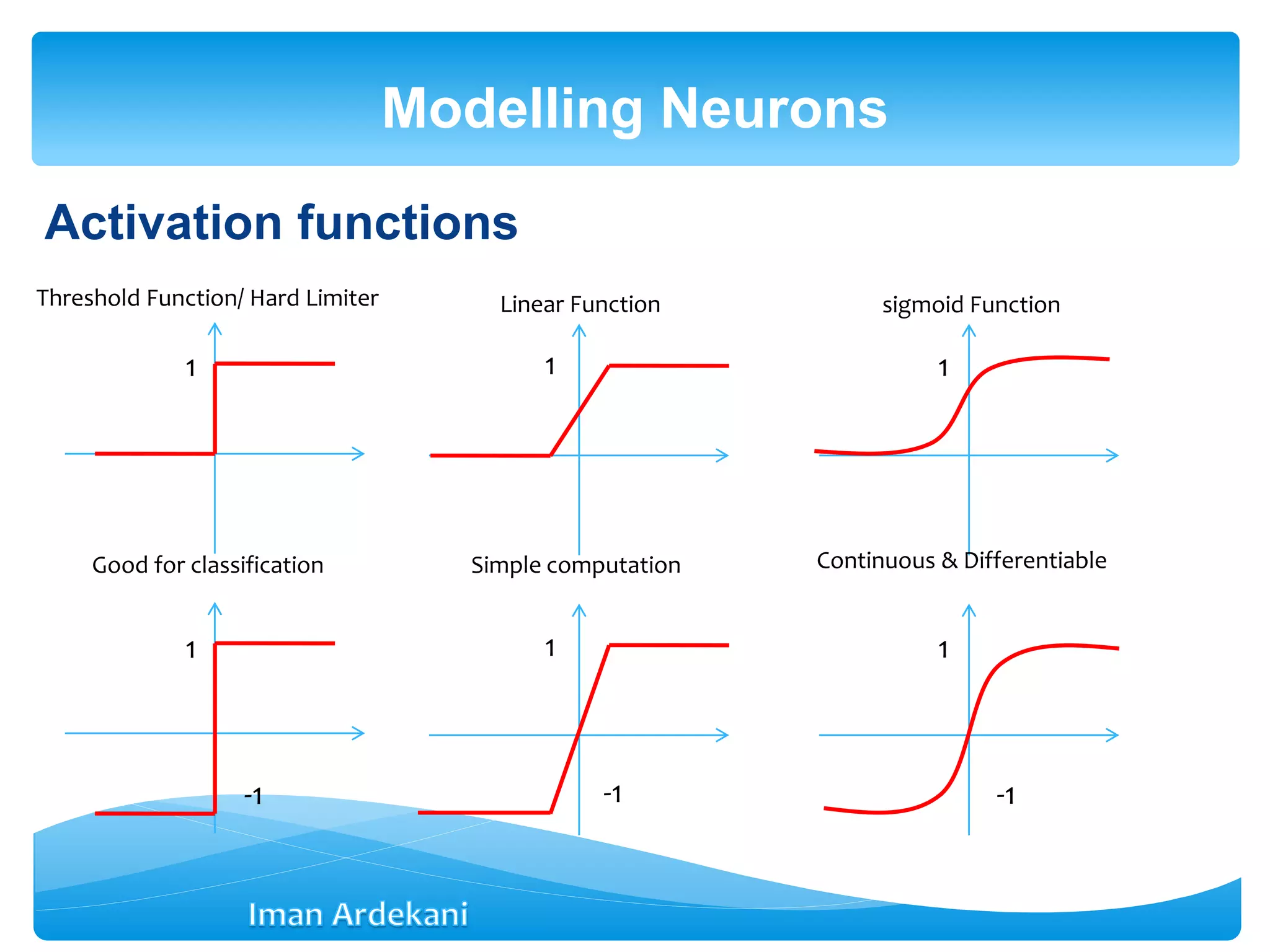
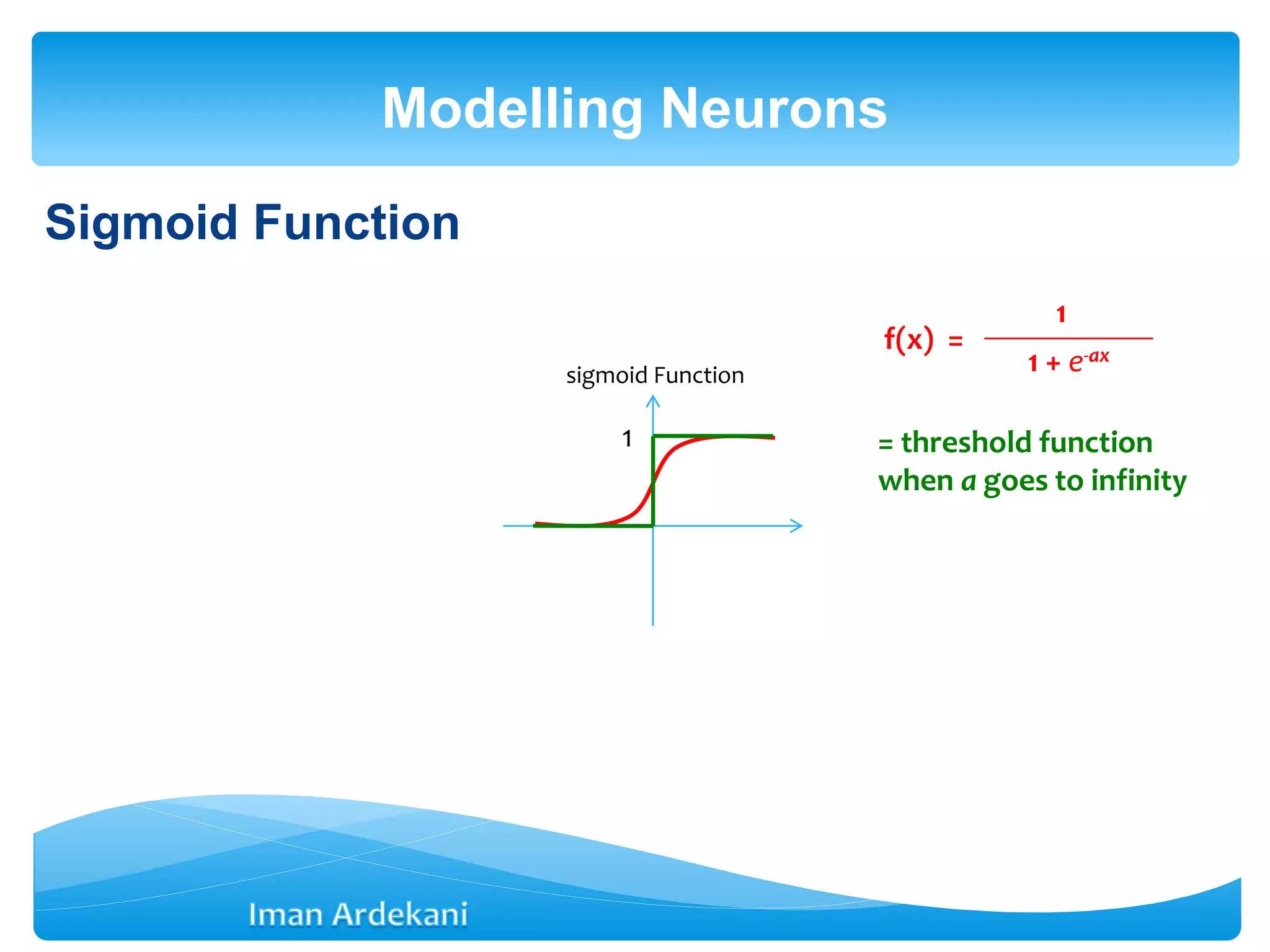
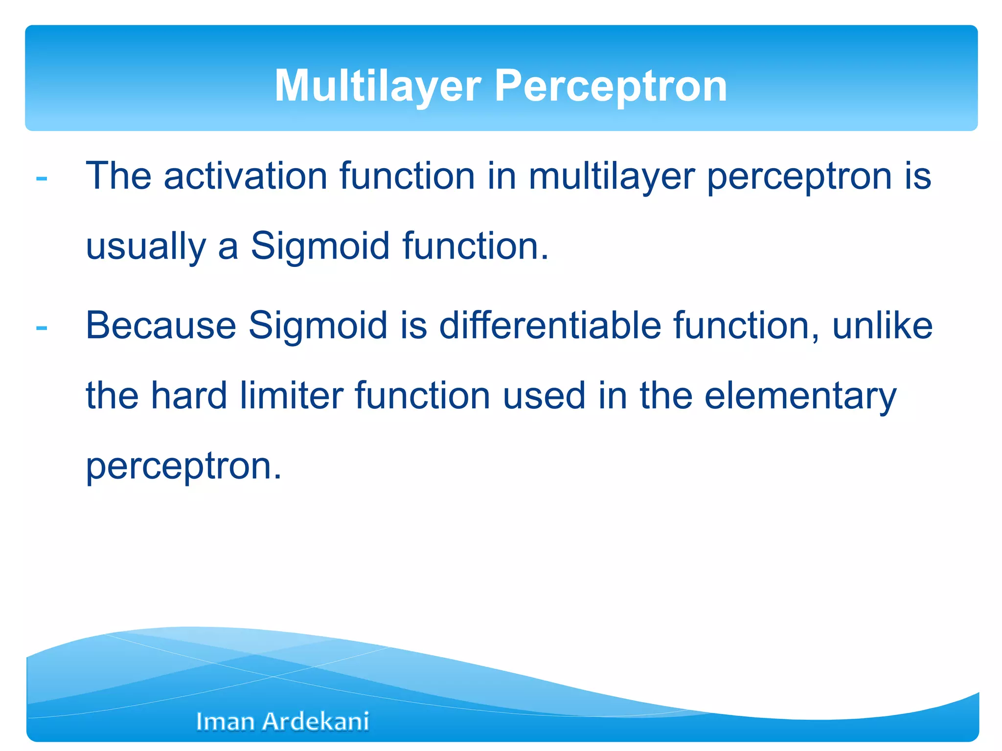
Each output is a function of the net stimulus signal (f is called the
activation function)
y = f (net) = f(b + WTX)
Modelling Neurons](https://image.slidesharecdn.com/week3bann-150512031518-lva1-app6892/75/Artificial-Neural-Network-10-2048.jpg)
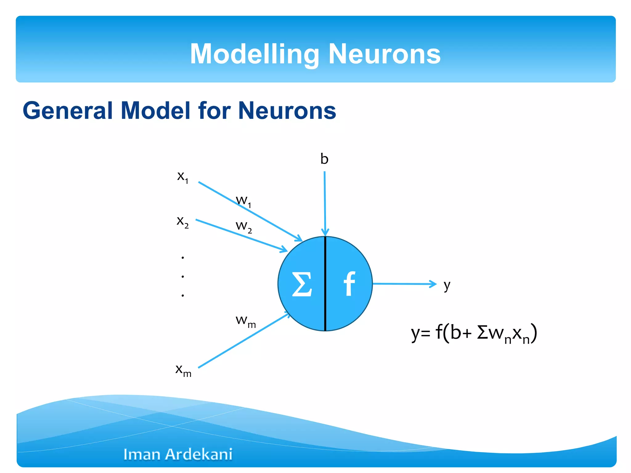
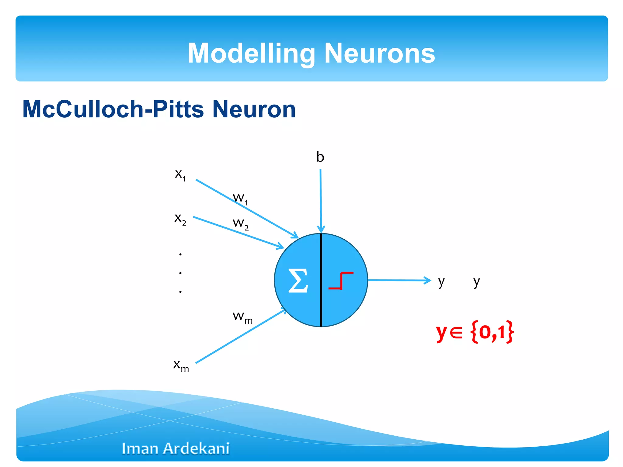
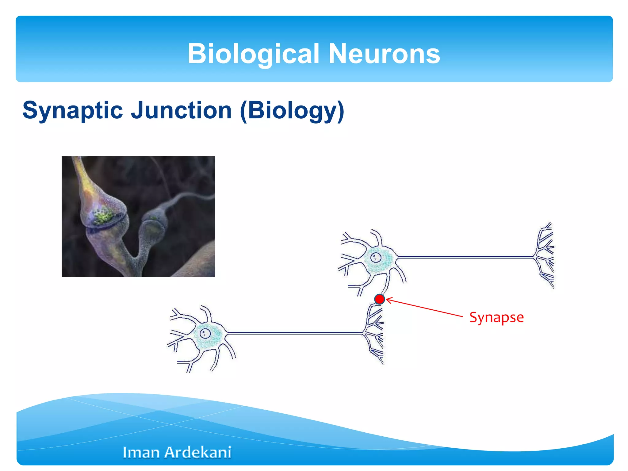
![Modelling Neurons
y [0,1]
x1
x2
xm
.
.
. y
w1
w2
wm
b](https://image.slidesharecdn.com/week3bann-150512031518-lva1-app6892/75/Artificial-Neural-Network-15-2048.jpg)


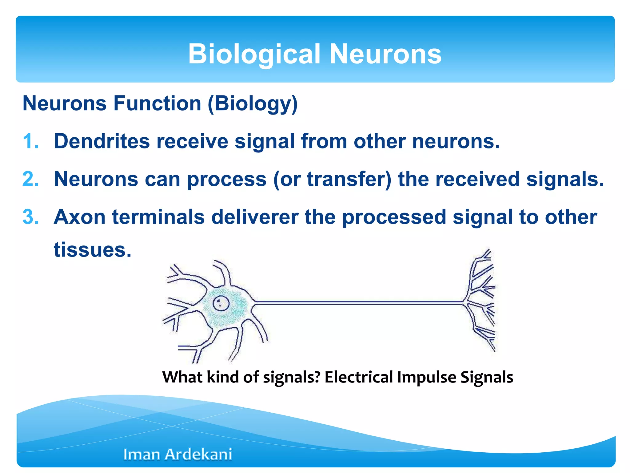
![Equivalent Presentation
Perceptron
x1
x2
xm
.
.
. y
w1
w2
wm
b
w0
1
net = WTX
Weight vector: W =[w0 w1 … wm]T
Input vector: X = [1 x1 x2 … xm]T](https://image.slidesharecdn.com/week3bann-150512031518-lva1-app6892/75/Artificial-Neural-Network-34-2048.jpg)
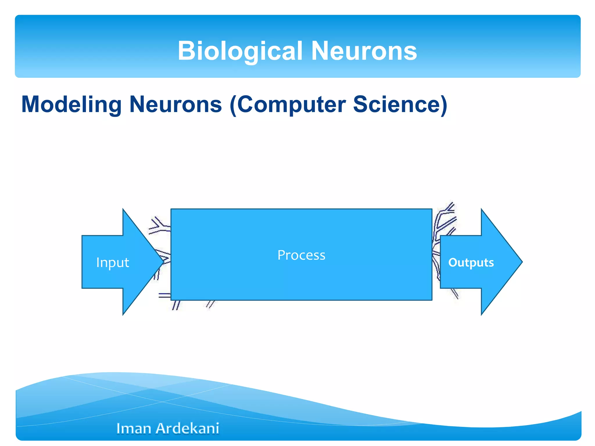
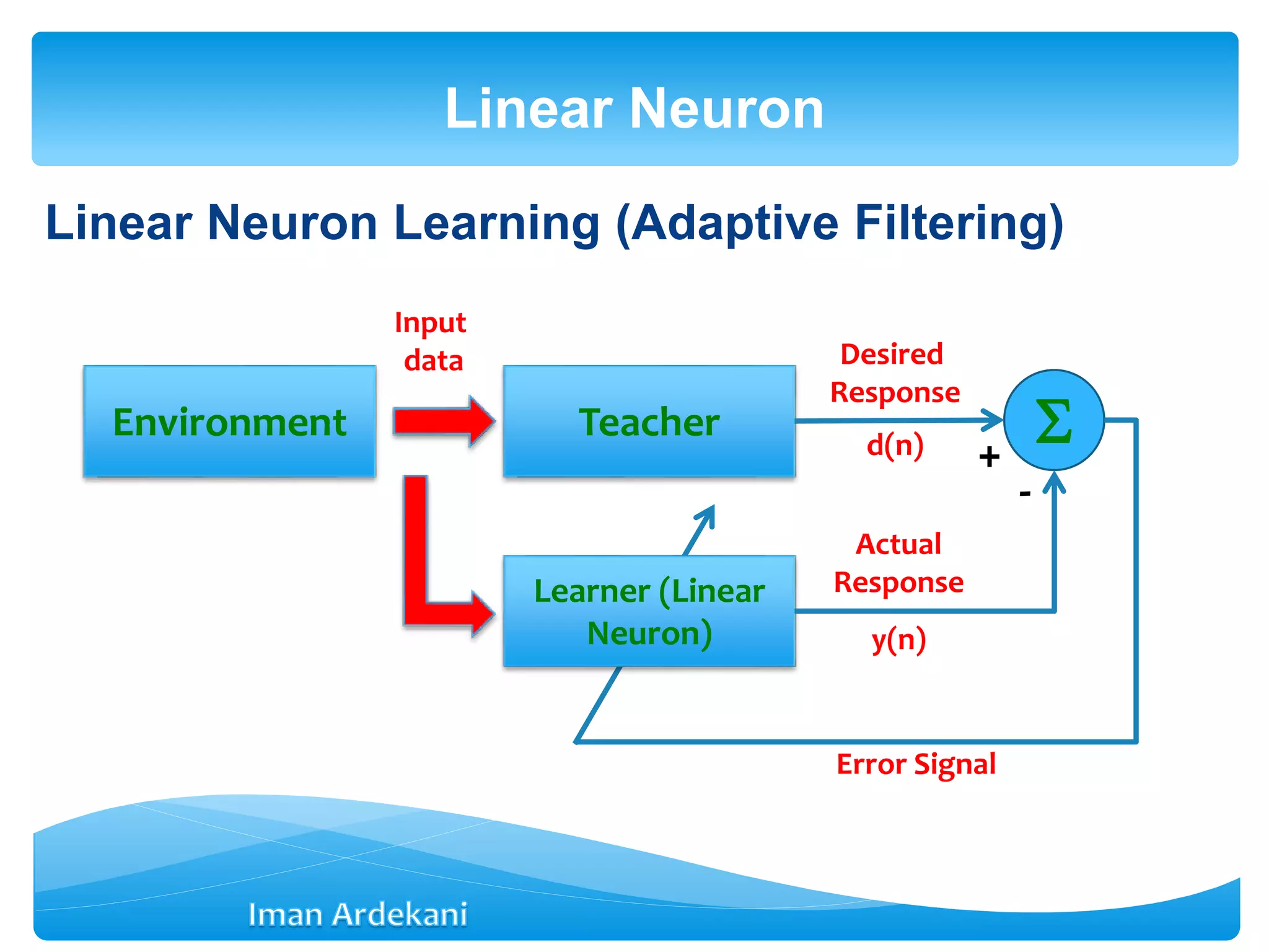
![- when the activation function simply is f(x)=x the
neuron acts similar to an adaptive filter.
- In this case: y=net=wTx
- w=[w1 w2 … wm]T
- x=[x1 x2 … xm]T
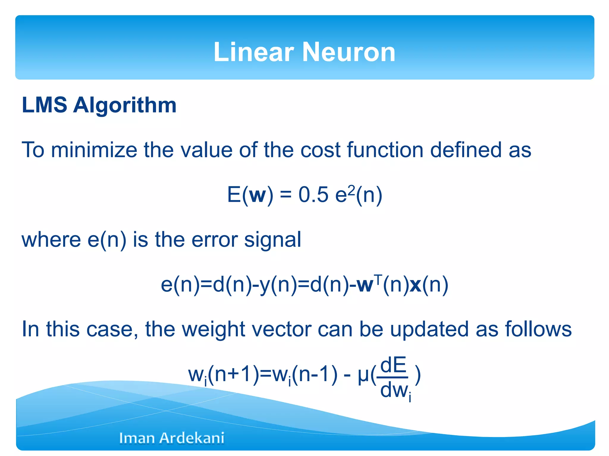
Linear Neuron
x1
x2
xm
.
.
. y
w1
w2
wm
b
](https://image.slidesharecdn.com/week3bann-150512031518-lva1-app6892/75/Artificial-Neural-Network-37-2048.jpg)
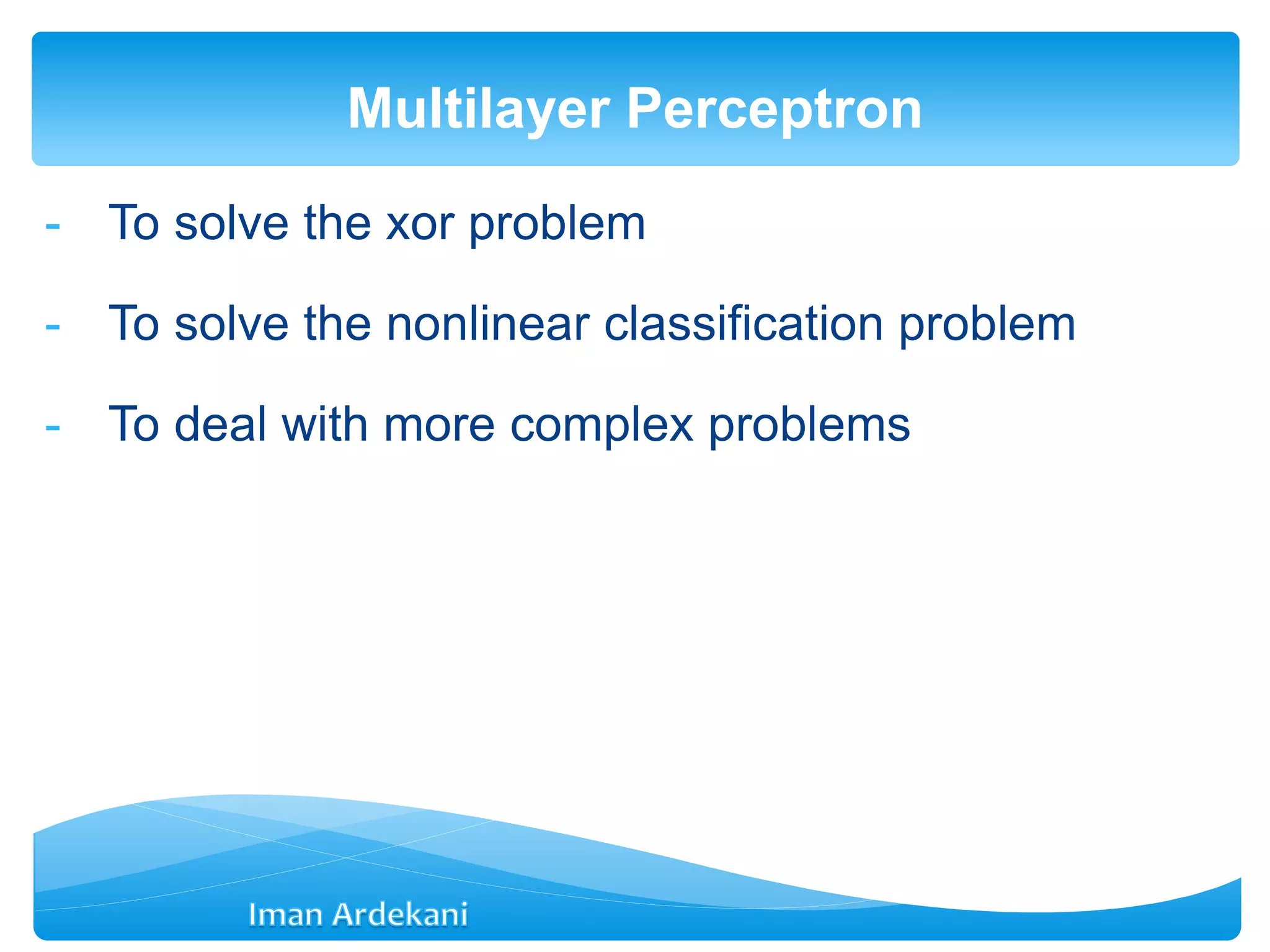
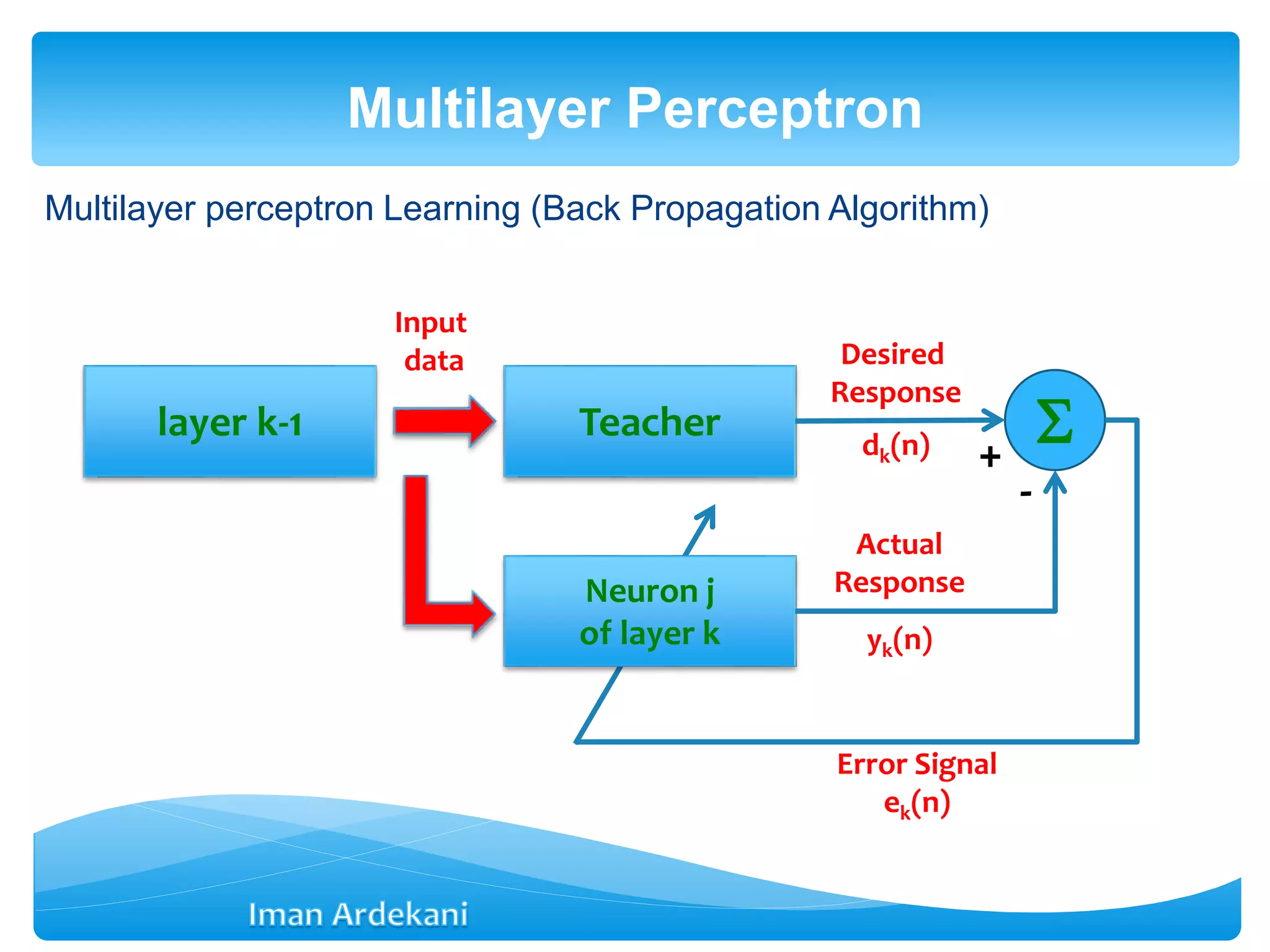
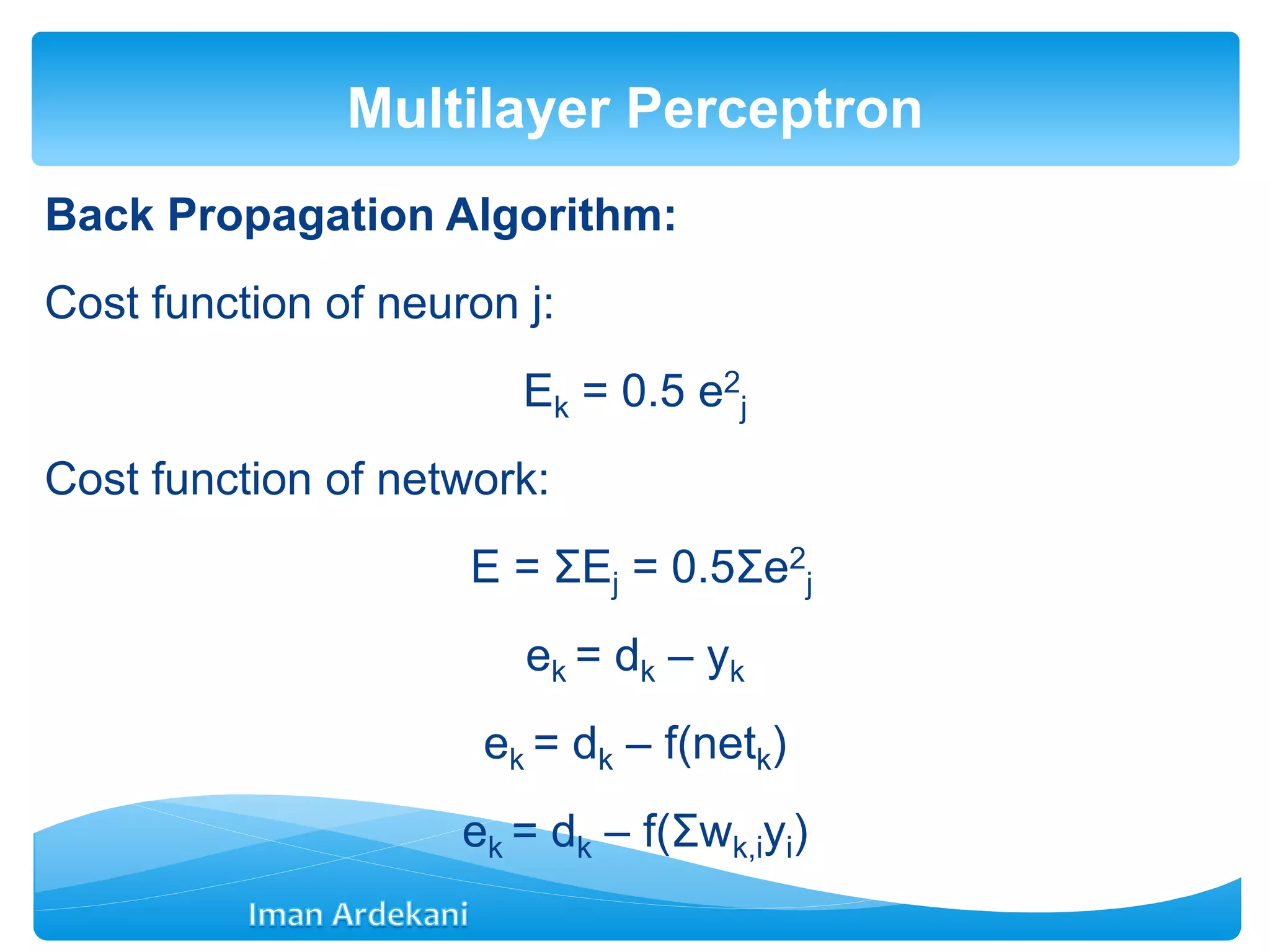
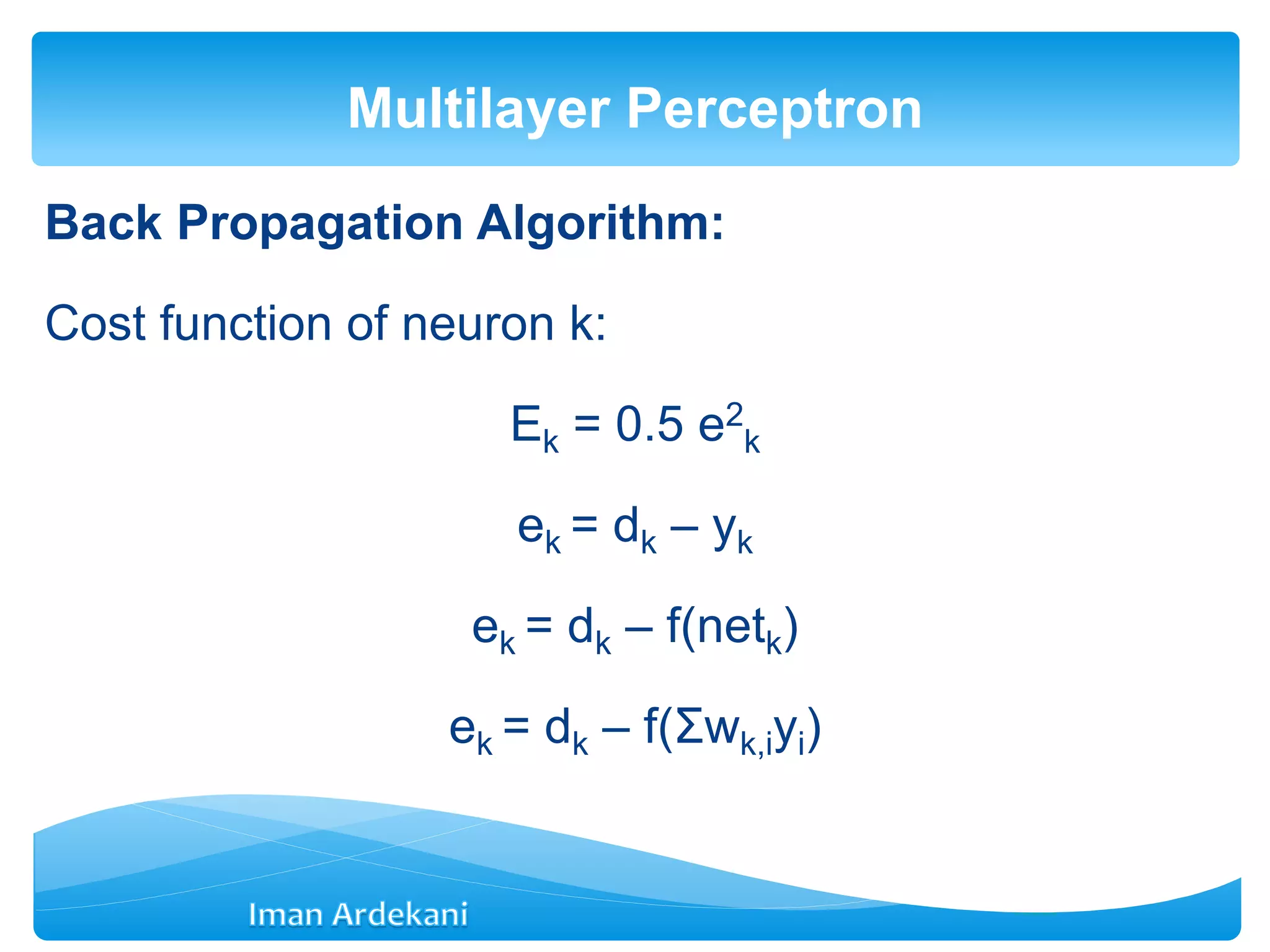
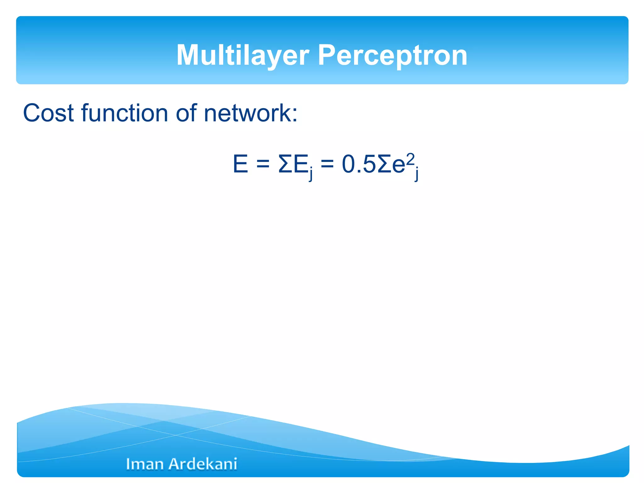
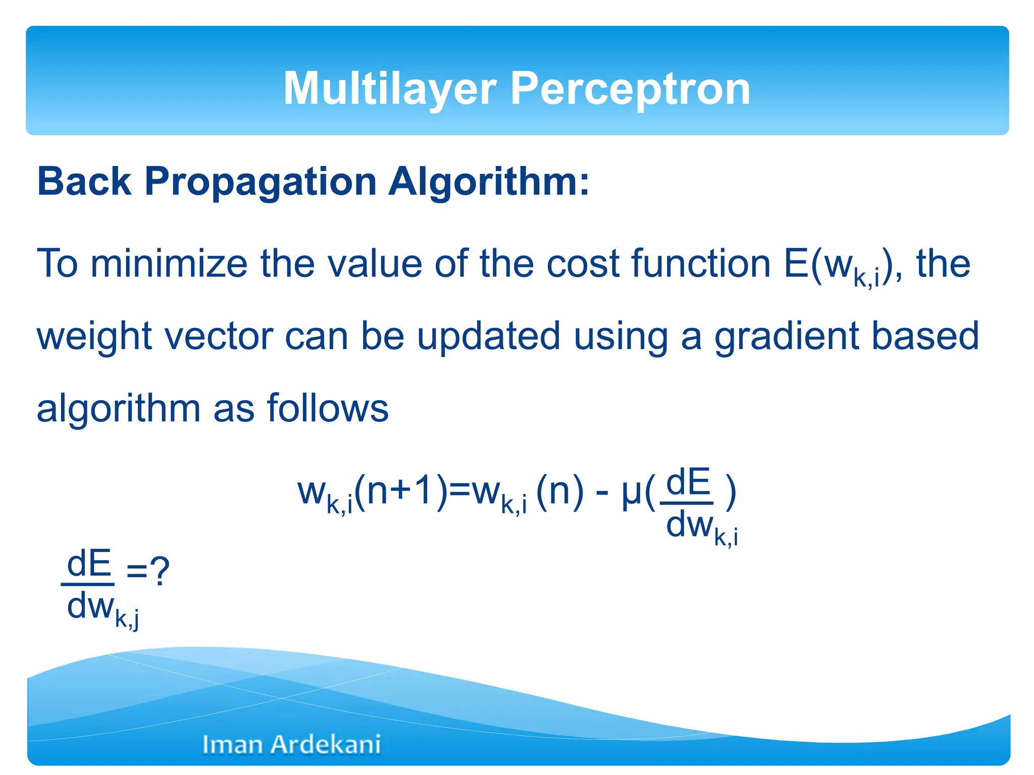
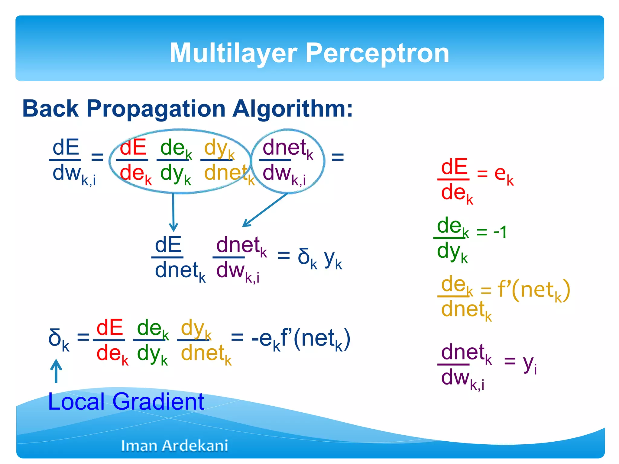
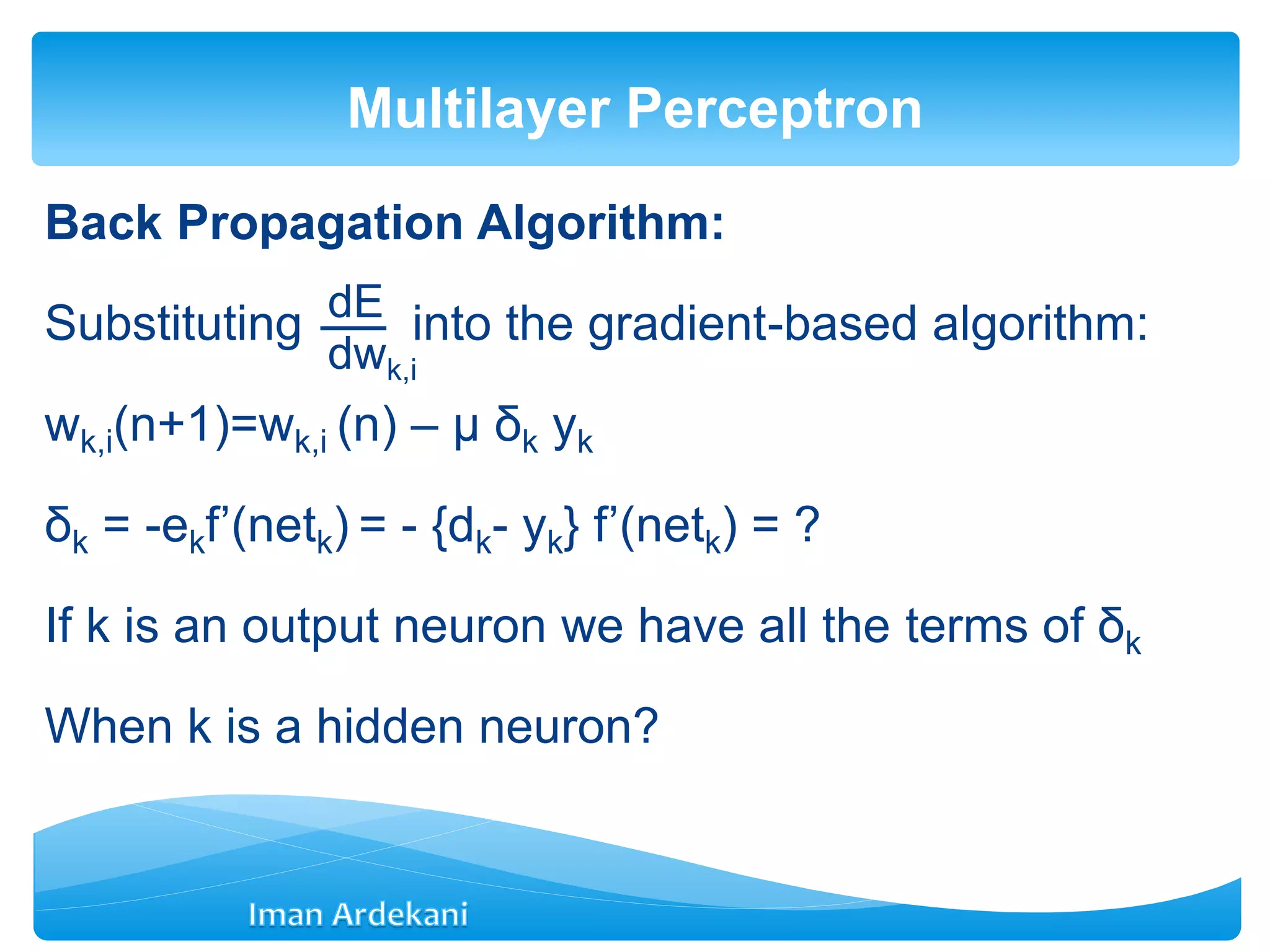
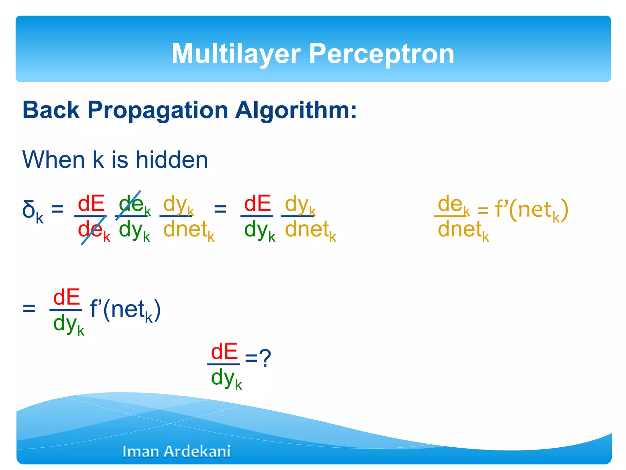
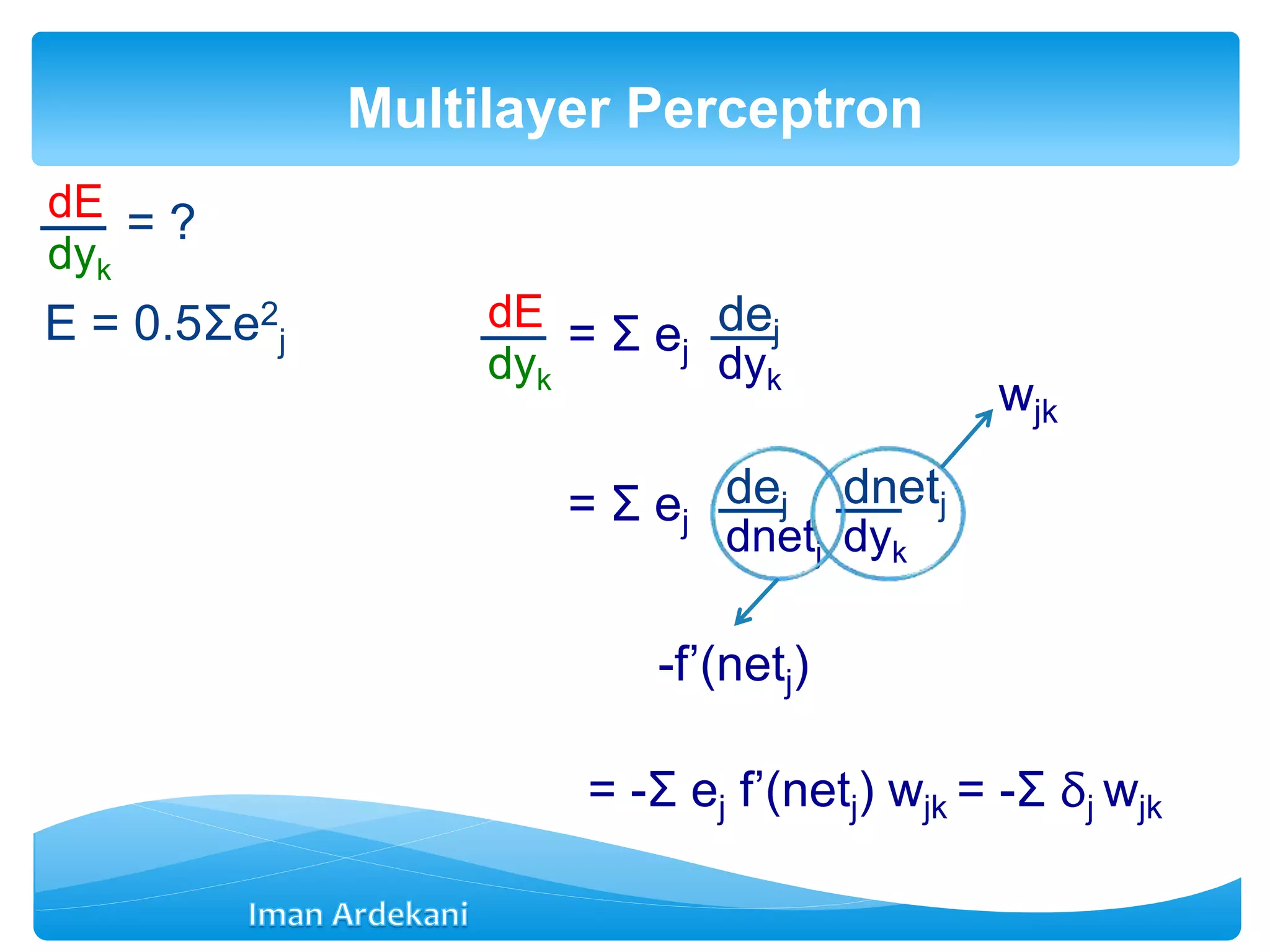

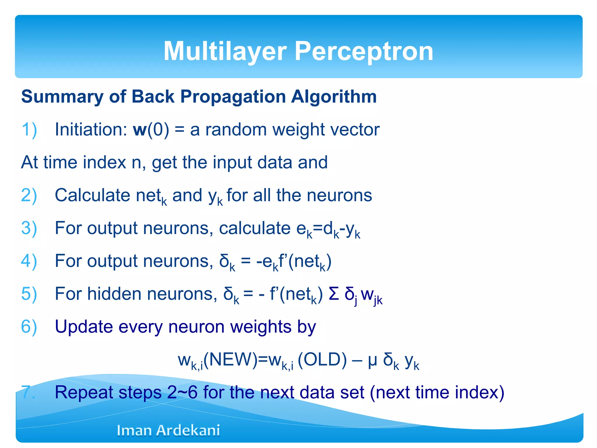


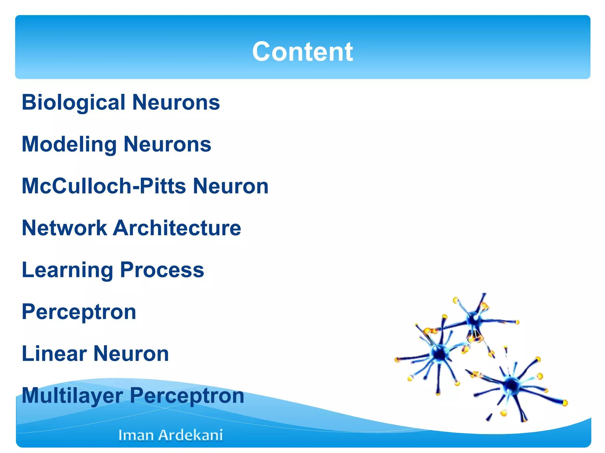
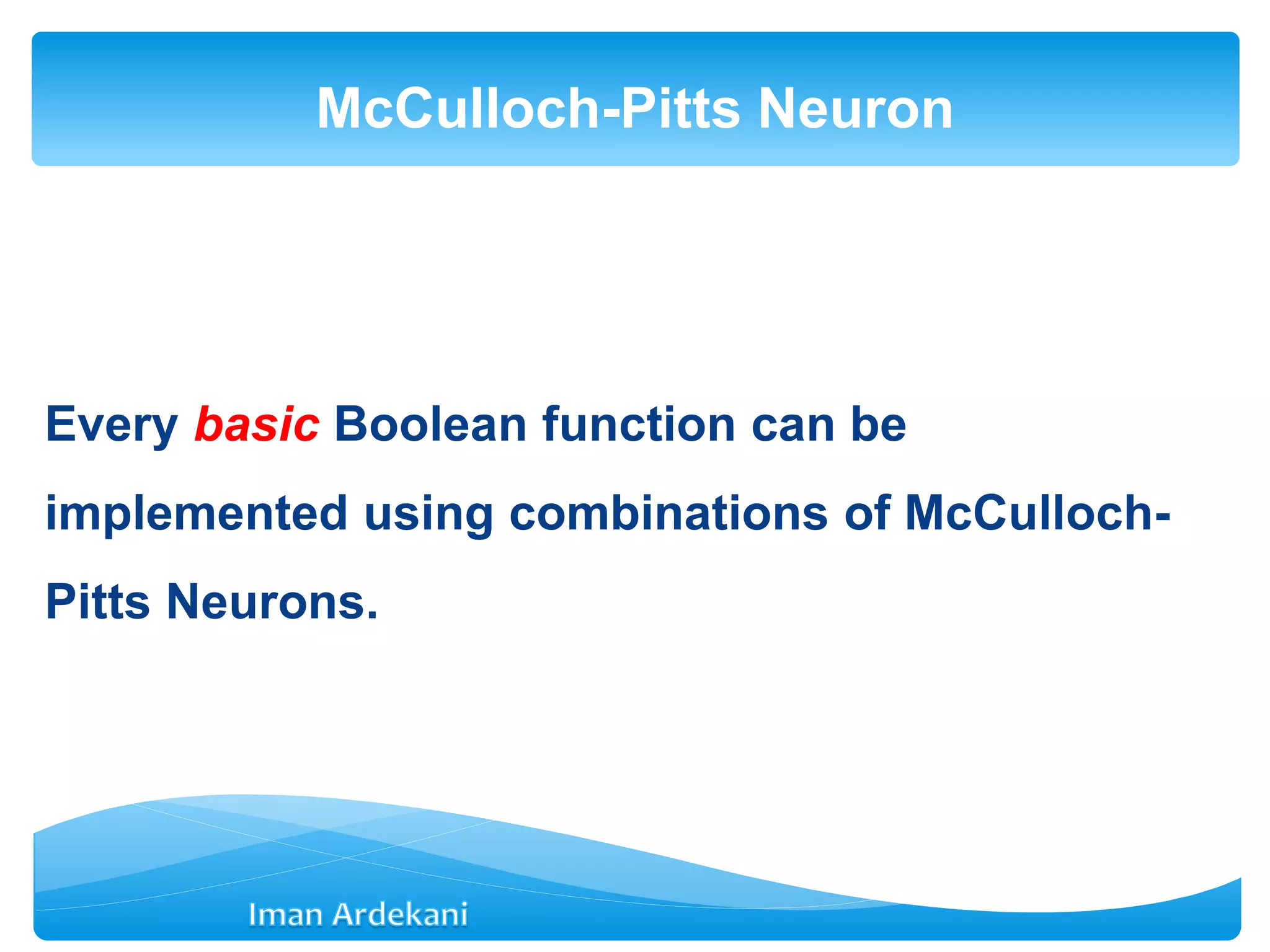
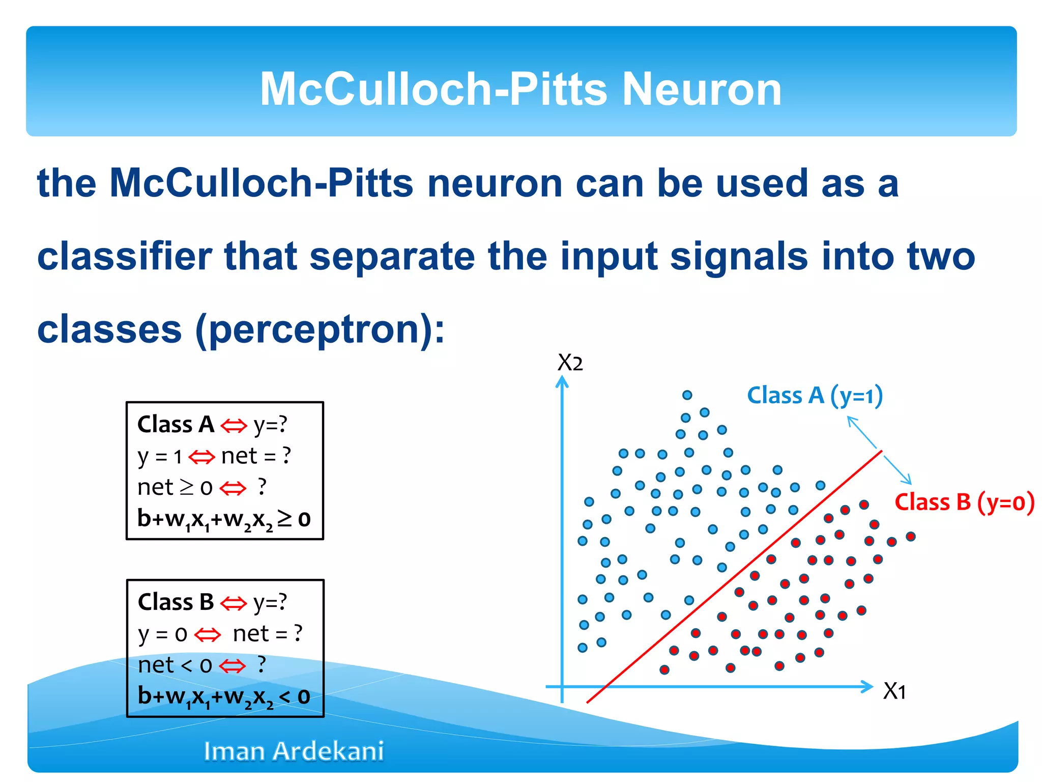
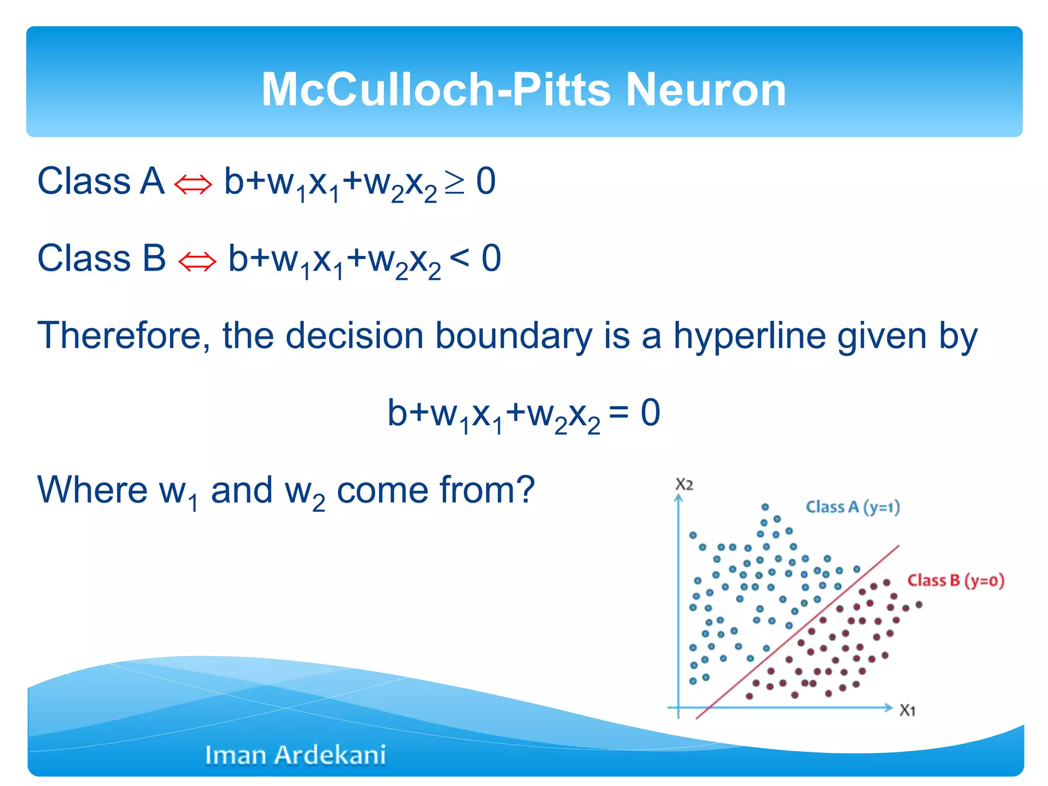
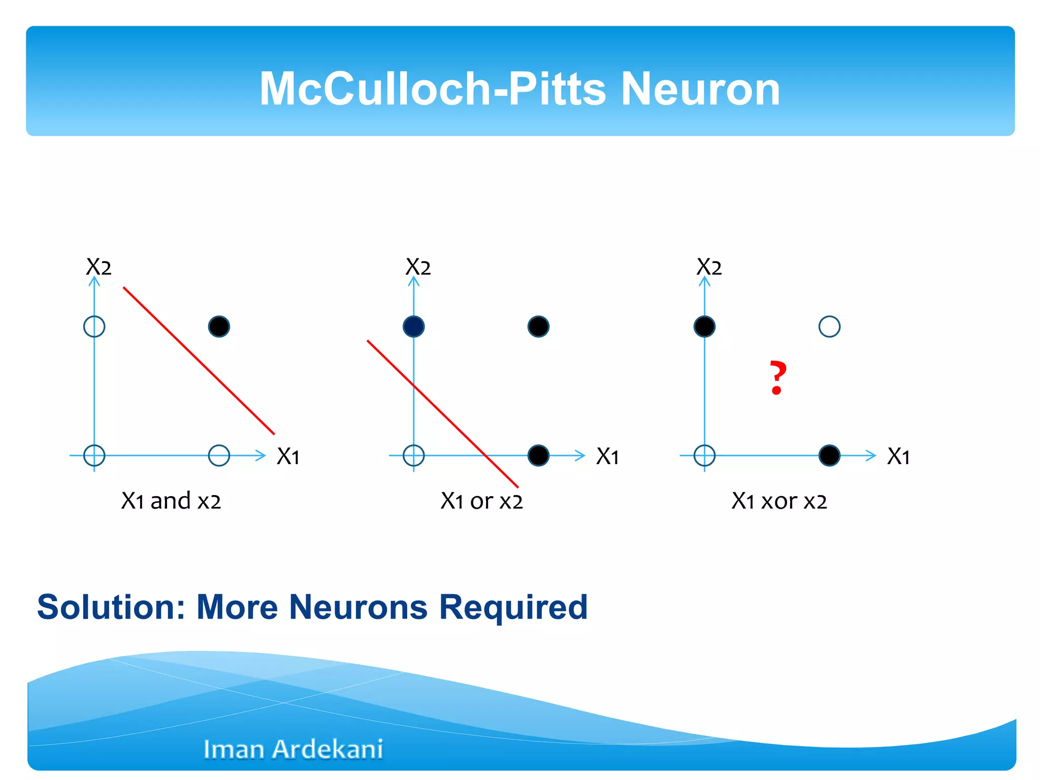
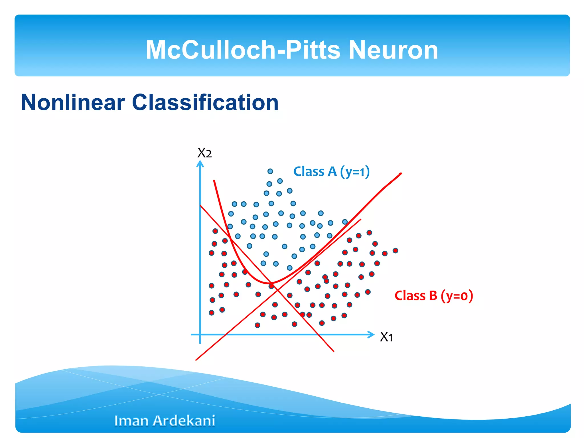
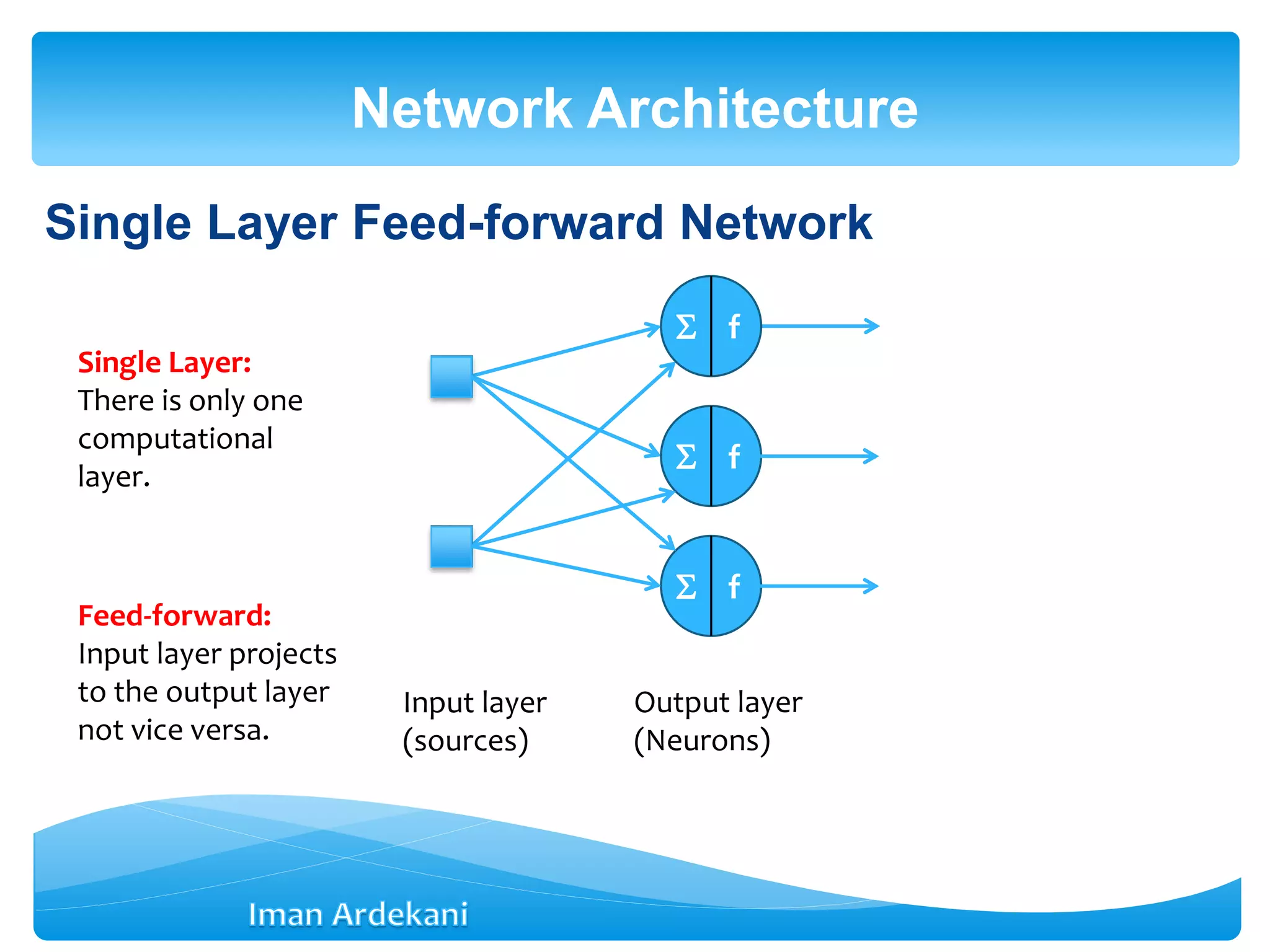
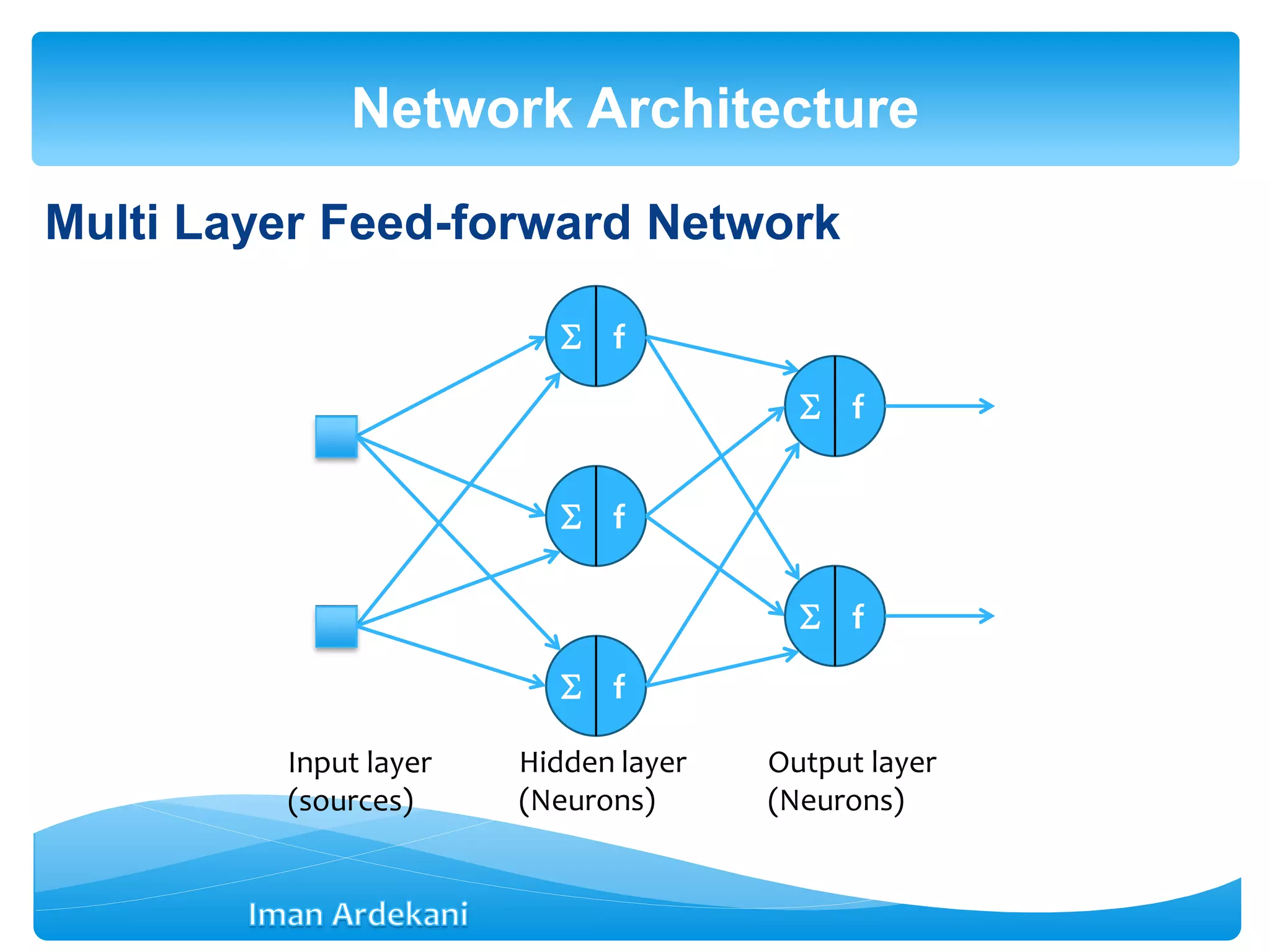
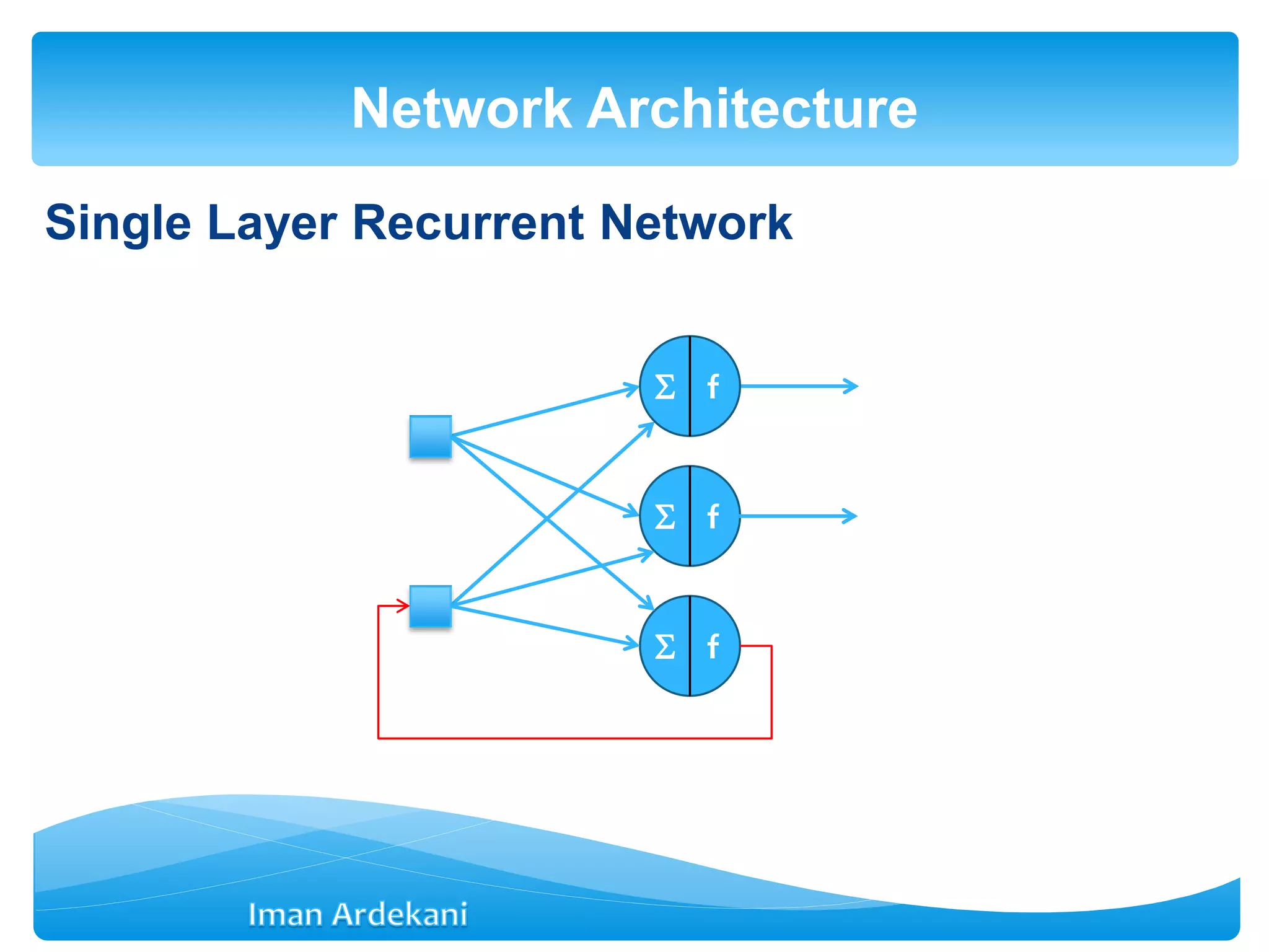
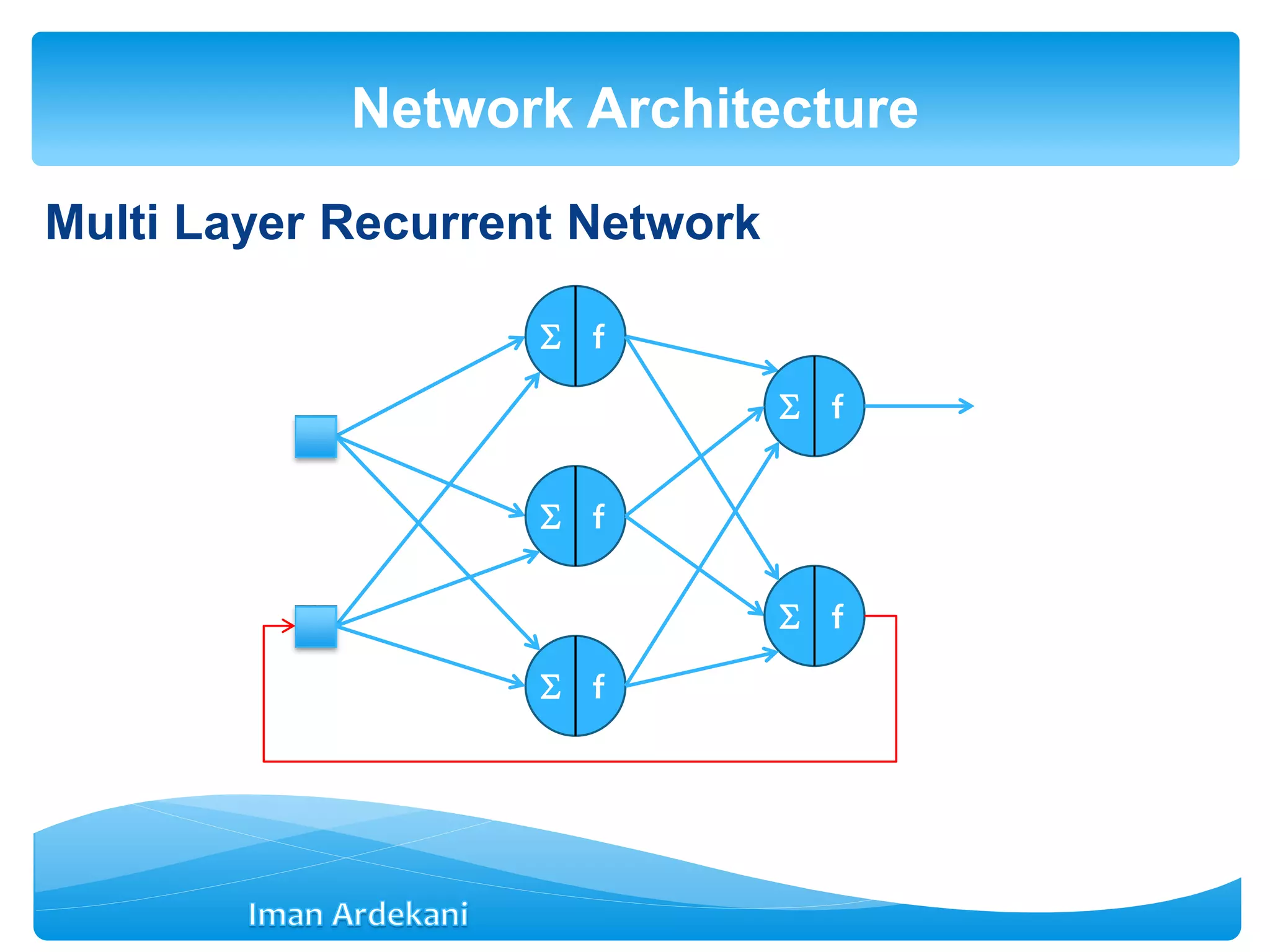
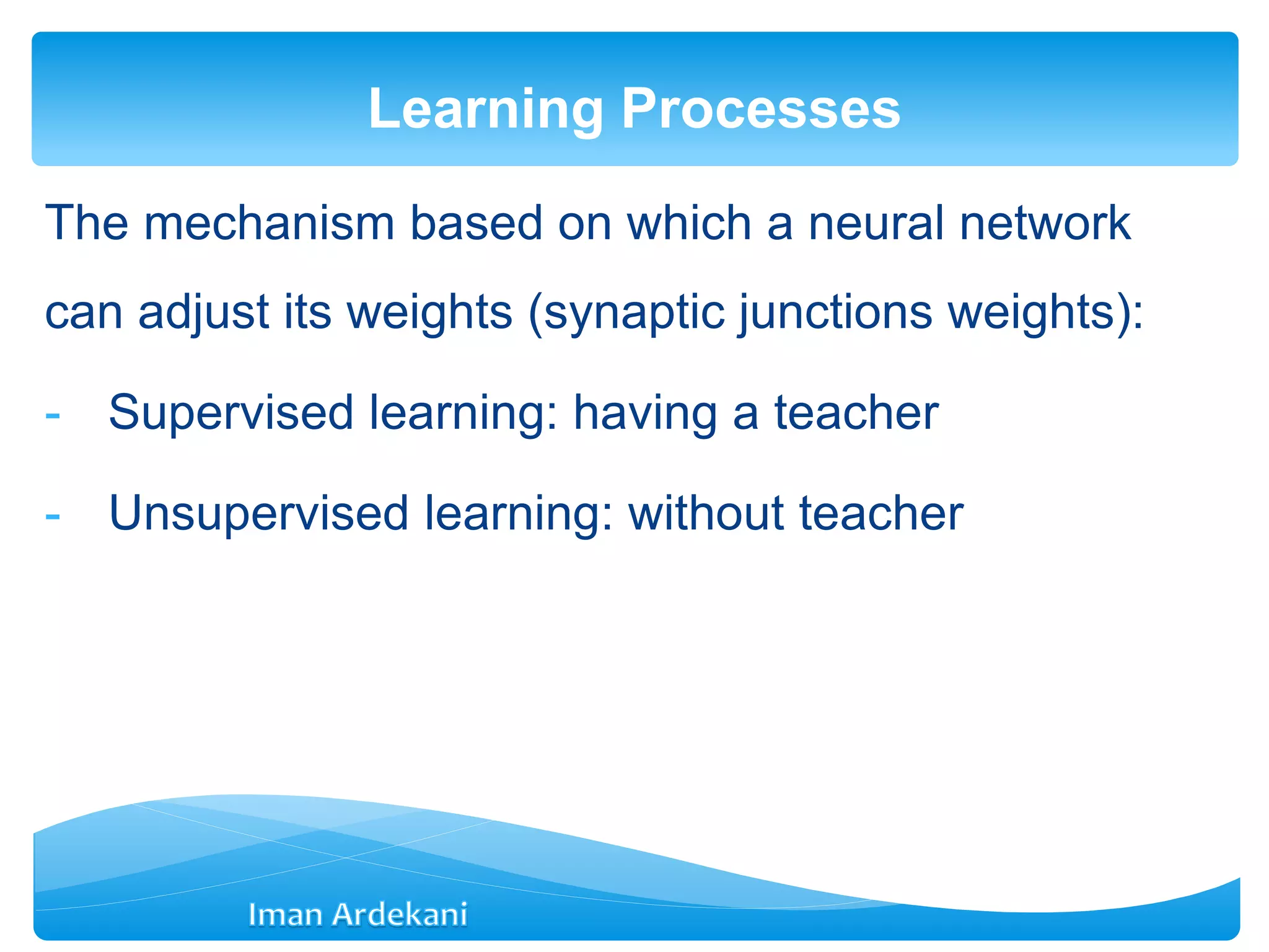
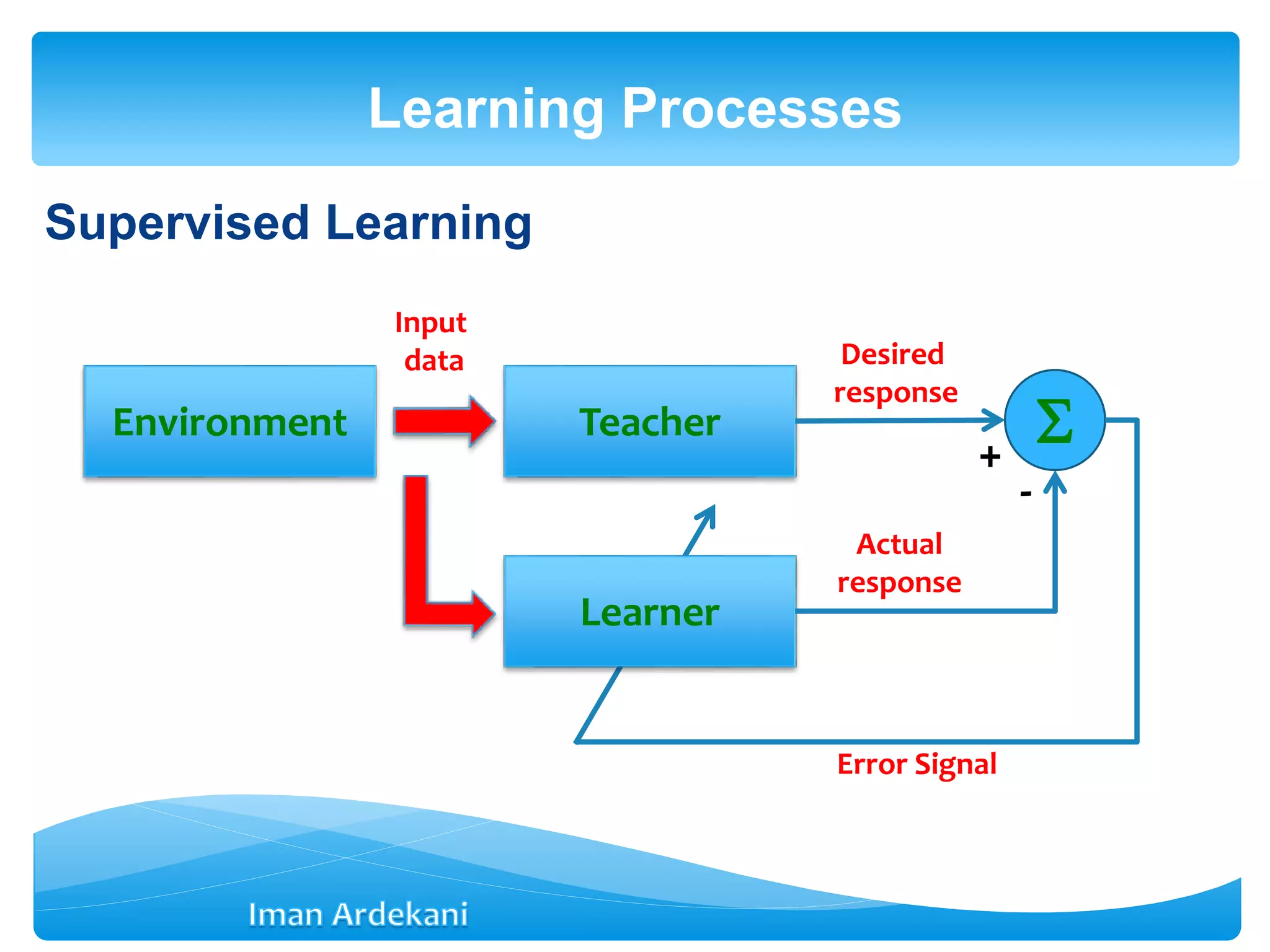
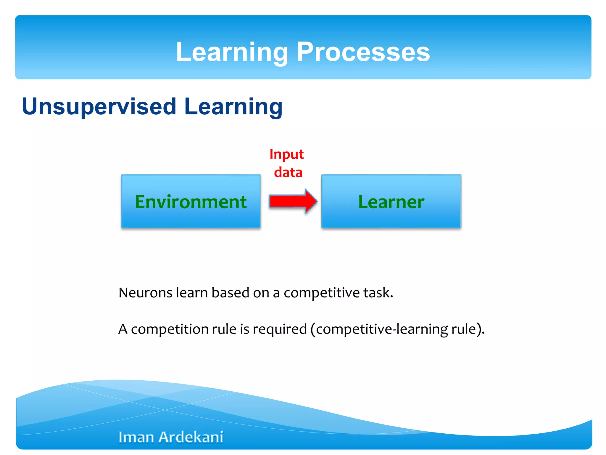
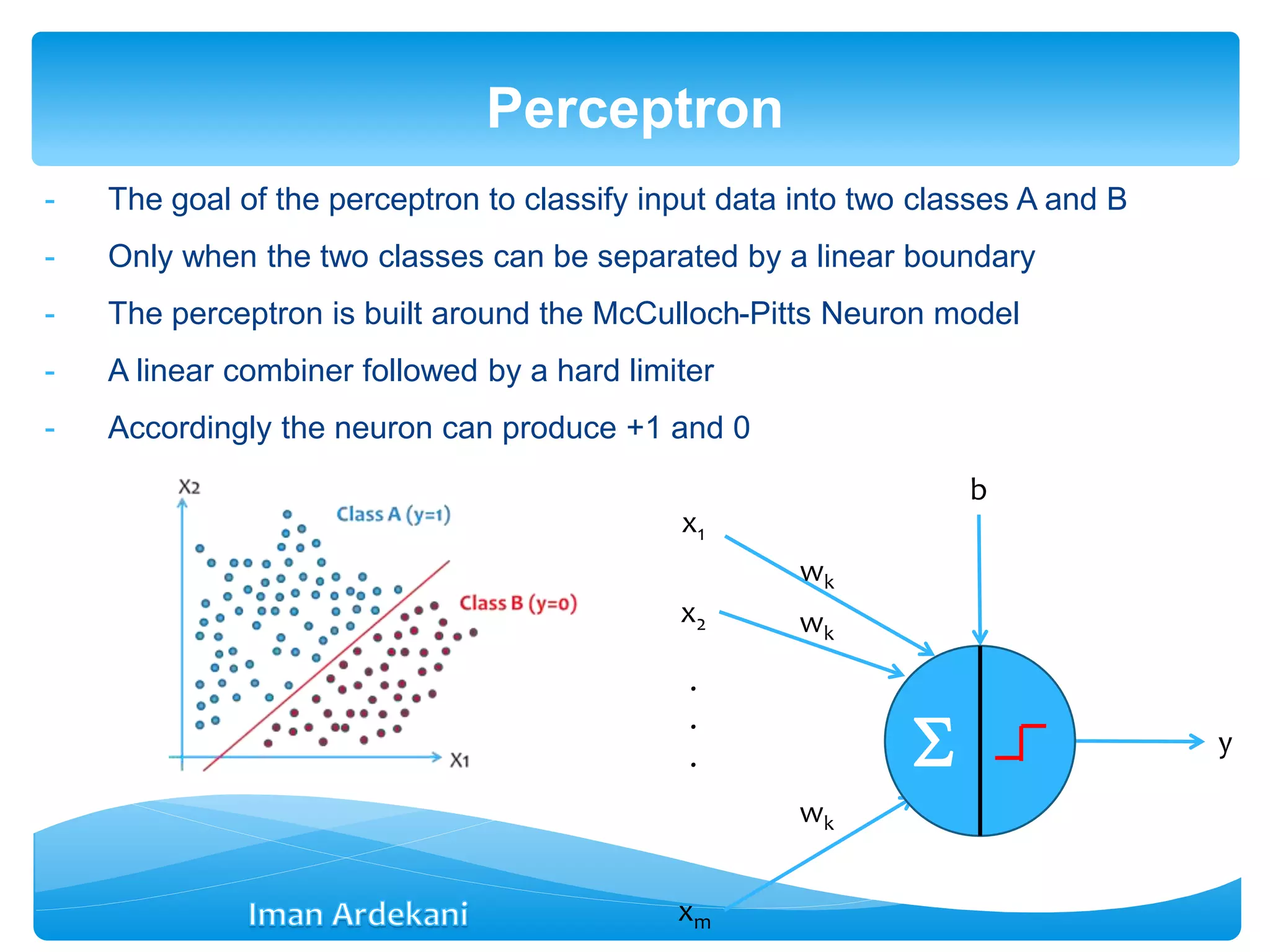
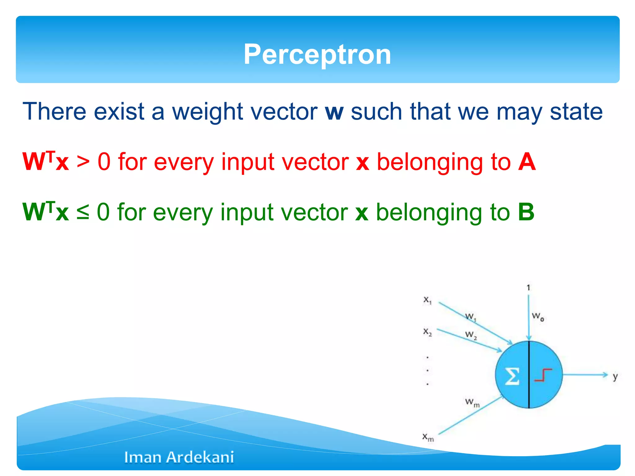
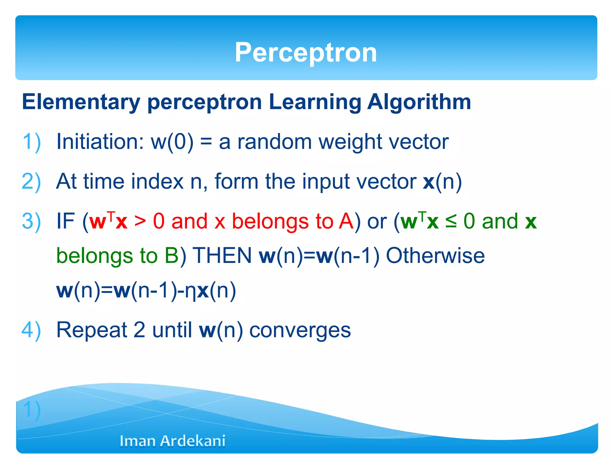
This document provides an overview of artificial neural networks. It discusses biological neurons and how they are modeled in computational systems. The McCulloch-Pitts neuron model is introduced as a basic model of artificial neurons that uses threshold logic. Network architectures including single and multi-layer feedforward and recurrent networks are described. Different learning processes for neural networks including supervised and unsupervised learning are summarized. The perceptron model is explained as a single-layer classifier. Multilayer perceptrons are introduced to address non-linear problems using backpropagation for supervised learning.