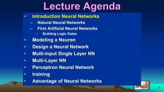
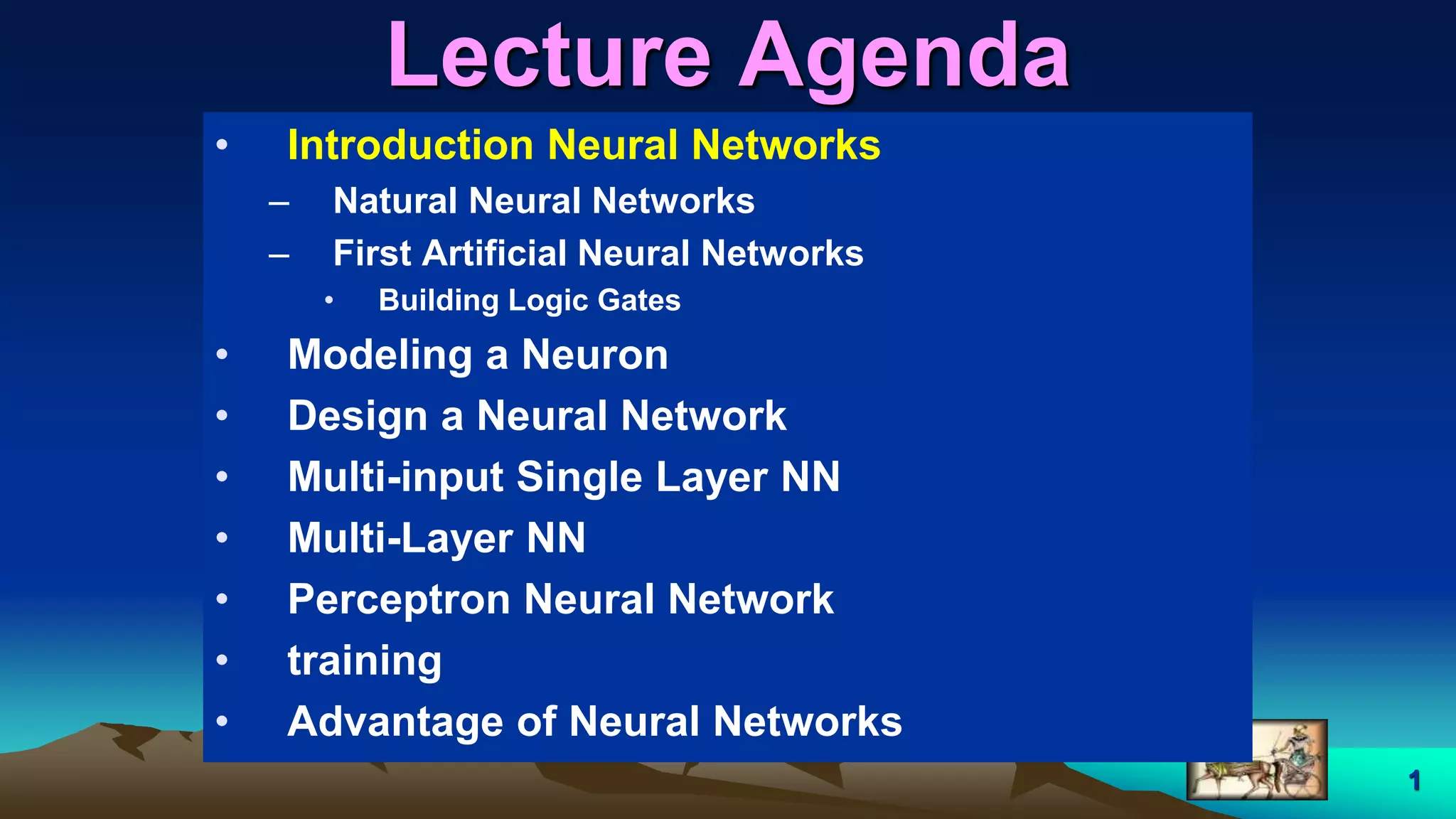
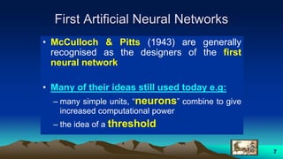
This document provides an overview of neural networks and related topics. It begins with an introduction to neural networks and discusses natural neural networks, early artificial neural networks, modeling neurons, and network design. It then covers multi-layer neural networks, perceptron networks, training, and advantages of neural networks. Additional topics include fuzzy logic, genetic algorithms, clustering, and adaptive neuro-fuzzy inference systems (ANFIS).

1. 1
Lecture Agenda
• Introduction Neural Networks
– Natural Neural Networks
– First Artificial Neural Networks
• Building Logic Gates
• Modeling a Neuron
• Design a Neural Network
• Multi-input Single Layer NN
• Multi-Layer NN
• Perceptron Neural Network
• training
• Advantage of Neural Networks

2. 2
Reasoning Learning Optimization
Fuzzy Logic
(FL)
Neural Networks
(NN)
Genetic Algorithm
(GA)
AI

3. 3
Neural Networks
• As you read these words you are using Complex
Biological Neural Networks
• Work in parallel , so that it is very fast.
• We are born with about 100 billion neurons
• A neuron may connect to as many as 100,000
other neurons

4. 4
“If the brain were so
simple, that we could
understand it, then
we’d be so simple that
we couldn’t”
Lyall Watson

5. 5
Axon from another cell
Nucleus
Axon
Soma or Cell body
Synapse
Synapses
Dendrite
Axonal arborization
Natural Neural Networks

6. 6
Neural Networks
• Signals “move” via electrochemical signals
• The synapses release a chemical
transmitter – the sum of which can cause a
threshold to be reached – causing the
neuron to “fire”
• Synapses can be inhibitory or excitatory

7. 7
First Artificial Neural Networks
• McCulloch & Pitts (1943) are generally
recognised as the designers of the first
neural network
• Many of their ideas still used today e.g:
– many simple units, “neurons” combine to give
increased computational power
– the idea of a threshold

8. 8
Building Logic Gates
• Computers are built out of “logic gates”
• Can we use neural nets to represent logical functions?
• Use threshold (step) function for activation function
– all activation values are 0 (false) or 1 (true)

9. 9
The First Neural Neural
Networks
AND
X1 X2 Y
1 1 1
1 0 0
0 1 0
0 0 0Threshold(Y) = 2
AND Function
1
1X1
X2
Y
Threshold(Y) = 2
inputs weights outputs

10. 10
The First Neural Neural
Networks
AND Function
OR Function
2
2X1
X2
Y
OR
X1 X2 Y
1 1 1
1 0 1
0 1 1
0 0 0
Threshold(Y) = 2

11. 11
The First Neural Neural
Networks
AND
NOT
X1 X2 Y
1 1 0
1 0 1
0 1 0
0 0 0
Threshold(Y) = 2
AND NOT Function
-1
2X1
X2
Y

12. 12
Modeling a Neuron
• aj :Activation value of unit j
• wi,j :Weight on the link from unit j to unit i
• ini :Weighted sum of inputs to unit i
• ai :Activation value of unit i
• g :Activation function
 j
jjii aWin ,
Wi,j

13. 13
Example 1: (Matlab based)
• NN parameters are: w’s, b’s, f’s
w11
INPUTS TARGET
∑w12
P1
P2
-1
5 b1
1
23
2
f(n)
an
Single layer 2 inputs 1 output Neural Networks
P1, P2: inputs
w11, w12: weight
b1: bias
n: activation
f: transfer function
a: actual output
T: target
error: T – a
a= f(n)
a= f( P1* w11 + P2* w12 + b1 )
f: let it pure linear
2*-1 + 3*5 + 2*1 = 15
n= 15
T

14. 14
Design a Neural Network
• Is to select the best:
– w’s weights,
– b’s biases,
– and f transfer function (selection will be based
on the problem you are studying.)
which make the error as low as possible.
• Which can be chosen and trained
 automatically using matlab.

15. 15
Type of functions:
1- Hardlim
Case
• n is –ve  O/P = 0
• n is +ve or zero  O/P = 1
2- Hardlims
Case
• n is –ve  O/P = -1
• n is +ve or zero  O/P = 1
f(n)
?
an
a = hardlims(n)

16. 16
3- Purelin
• a = n
Type of functions:
a = n
f(n)
?
an
Note:
What ever you want in your linear system
Can be done before this purelin.
Ex: If you want 2*(input) +1
weight w bias b

17. 17
4. Logsig
– a = 1/ (1 + exp(-n) )
5. Tansig
– a = (exp(n) – exp(-n)) / (exp(n) + exp(-n))
Type of functions:
f(n)
?
an

18. 18
Multi-input Single Layer NN
.
w11
INPUTS
w12
P1
P2
b1
f(n)
a1n1 q: number of inputs
S1: number of neurons
in the 1st layer
Pq
.
.
.
.
w1q
b2
f(n)
a2n2
b3
f(n)
a3n3
.
.
.
.
S1
Layer 1
w21
w22
w2q
w31
w32
w3q
W(to where)(from where)
In the same layer there is only
one type of transfer function f
)...(
)...(
22222112
11221111
bwPwPfa
bwPwPfa


)( 111 111   SSS bPWfa qq
...)......(......  f

19. 19
)( 111 111   SSS bPWfa qq
qSqSS
q
q
q
ww
wwww
wwww
W

















1
11
1
.........
...............
...
...
1
2232221
1131211
S
1
2
1
1
1
1
1
...
















SS
S
b
b
b
b

20. 20
Multi-Layer NN
.
w11
INPUTS
w12
P1
P2
b1
f(n)
a’1n1
Pq
.
.
.
.
w1q
b2
f(n)
a’2n2
b3
f(n)
a’3n3
.
.
.
.
S1
Layer 1
w21
w22
w2q
w31
w32
w3q
w11
w12
a’1
a’2
b1
f(n)
a1n1
a’s1
.
.
.
.
w1S1
b2
f(n)
a2n2
b3
f(n)
a3n3
.
.
.
.
S2
Layer 2
w21
w22
w2S1
w31
w32
w3q

21. 21
P1
P2
.
.
.
.
.
Pq
qx1
1
bS1x1
WS1xq
f1 aS1x1
WS2xS1
1
bS2x1
f2
aS2x1
Layer 1 Layer 2
))((
)(
)2(
1
)1(
11
)1(
1
)2(
21
1121
211122
21122




SSSSSS
SSSSS
bbPWfWfa
baWfa
qq

22. 22
Perceptron Neural Network
• Synonym for Single-
Layer, Feed-Forward
Network
• First Studied in the 50’s
• Other networks were
known about but the
perceptron was the only
one capable of learning
and thus all research was
concentrated in this area
Wi,jIj W1,j

23. 23

24. 24

25. 25

26. 26

27. 27
Hard limit Perceptrons
• Definition
– Perceptron generated great interest due to its ability
to generalize from its training vectors and learn
from initially randomly distributed connections.
Perceptrons are especially suited for simple problems
in pattern classification.
– They are fast and reliable networks for the problems
they can solve.
w11
INPUTS TARGET
w12
P1
P2
b1
1
an 0
1
hardlim

28. 28
What can perceptrons represent?
0,0
0,1
1,0
1,1
0,0
0,1
1,0
1,1
• Functions which can be separated in this way are called
Linearly Separable
• Only linearly Separable functions can be represented by a
perceptron

29. 29
What can perceptrons represent?
Linear Separability is also
possible in more than 3
dimensions – but it is harder
to visualize

30. 30
.
w11
INPUTS TARGET
w12
P1
P2
b1
1
an 0
1
hardlim
12
1
1
12
11
2
1212111
'0
w
b
P
w
w
P
boundarythesthisnwhen
bPwPwn



n<0
a=0
P1
P2
slopeline
slopelinearpependicul
1

11
12
w
w
12
1
w
b

n>0
a=1
n=0
a=1
11
1
w
b


31. 31
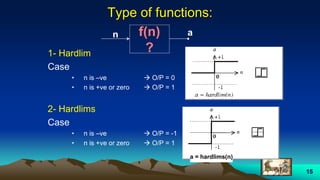
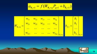
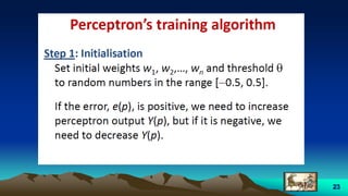
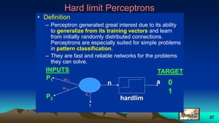
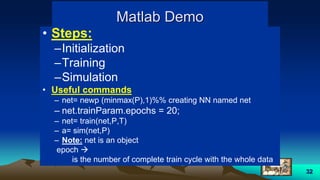
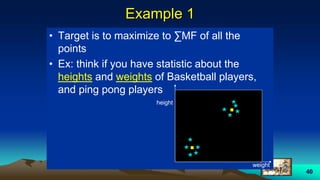
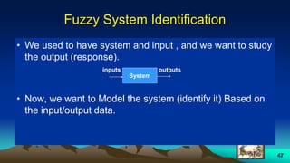
Example 2
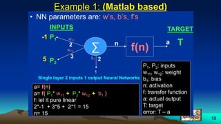
• P1 = [2 -2 4 1];
• P2 = [3 -5 6 1];
• Target:
– T= [1 0 1 0];
• We want:
– The Decision line
• Note:
– We must have linearly
separable data
*
*
o
P2
P1
o - 5
- 2 2
3
6
4
*
*o
P2
P1
o
Not linearly
Separable data

32. 32
Matlab Demo
• Steps:
–Initialization
–Training
–Simulation
• Useful commands
– net= newp (minmax(P),1)%% creating NN named net
– net.trainParam.epochs = 20;
– net= train(net,P,T)
– a= sim(net,P)
– Note: net is an object
epoch 
is the number of complete train cycle with the whole data

33. 33
Training
Patch
training
Adaptive
training

34. 34
Function: train
Algorithm:
• train calls the function indicated by net.trainFcn,
using the training parameter values indicated by
net.trainParam.
• Typically one epoch of training is defined as a
single presentation of all input vectors to the
network. The network is then updated according
to the results of all those presentations.
• Training occurs until :
– a maximum number of epochs occurs
– the performance goal is met
– The maximum amount of time is exceeded.
– or any other stopping condition of the function
net.trainFcn occurs.

35. 35
Classification Capability of Perceptrons
• 1 neuron {0,1}  2 possibilities
• 2 neurons { (0,0),
(0,1),
(1,0),
(1,1) }  4 possibilities
• N neurons  2N possibilities

36. 36
Perceptrons
• If there is zero bias the line will pass the origin
• Against each pair of inputs (column) there is
one pair of outputs (column)
• The Line start with zeros weights and biases
 means the line will be horizontal.
• No need to use multi-layers of Perceptrons
– The algorithm is hard
– No reason we already have 0 or 1(so no need)

37. 37
Advantage of Neural Networks
• Learning ability
• Generalization (means even for new data)
• Massive potential parallelism
• Robustness (means, it will work even it has some
corrupted parts)

38. 38
Clustering
• Clustering of numerical data forms the basis
of many classification and system modeling
algorithms.
• The purpose of clustering: is to distill
natural groupings of data from a large data
set, producing concise representation of a
system’s behavior.

39. 39
Fuzzy Clustering (Fuzzy C means)
• Fuzzy c-means (FCM) is a data clustering
technique where each data point belongs to a
cluster to a degree specified by a membership
grade. This technique was originally introduced by
Jim Bezdek in 1981
• Target is to maximize to ∑MF of all the points

40. 40
Example 1
• Target is to maximize to ∑MF of all the
points
• Ex: think if you have statistic about the
heights and weights of Basketball players,
and ping pong players
** ***
*
*
*
**
.
.height
weight

41. 41
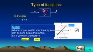
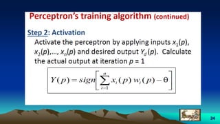
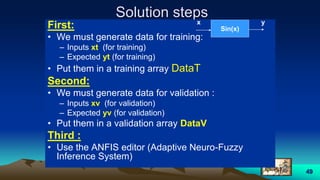
Example 1
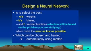
• x = [1 1 2 8 8 9];
• y = [1 2 2 8 9 8];
• axis([0 10 0 10]);
• hold on
• plot (x,y,’ro’);
• data= [x’ y’];
• c= fcm(data,2)%% data , number of groups
• plot (c(:,1), c(:,2), ‘b^’);

42. 42
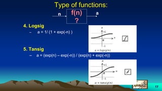
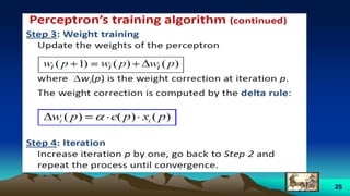
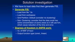
Example 2
• It is required to make the user to hit points
in x,y plan  using ginput
while(1)
[xp,yp]=ginput(1);
• Before that a message box would appear
to ask the user to input how many number
of clustering is required  using inputdlg
• Mark the clustering output

43. 43
Matlab Demo

44. 44
ANFIS
• ANFIS stands for Adaptive Neuro-Fuzzy Inference System.
(By Roger Jang 1993)
• Fundamentally, ANFIS is about taking a fuzzy inference
system (FIS) and tuning it with a backpropagation
algorithm based on some collection of input-output data.
• This allows your fuzzy systems to learn.
– A network structure facilitates the computation of the
gradient vector for parameters in a fuzzy inference system.
– Once the gradient vector is obtained, we can apply a number
of optimization routines to reduce an error measure (usually
defined by the sum of the squared difference between
actual and desired outputs).
• This process is called learning by example in the neural
network literature.

45. 45
ANFIS
• ANFIS only supports Sugeno systems subject to
the following constraints:
– First order Sugeno-type systems
– Single output derived by weighted average defuzzification
– Unity weight for each rule
• Warning:
– An error occurs if your FIS matrix for ANFIS learning does
not comply with these constraints.
– Moreover, ANFIS is highly specialized for speed and
cannot accept all the customization options that basic
fuzzy inference allows, that is, you cannot make your
own membership functions and defuzzification functions;
you’ll have to make do with the ones provided.

46. 46
A hybrid neural net (ANFIS architecture) which is computationally
equivalent to Tsukomato’s reasoning method.
Layer1: membership functions, degree of satisfaction
Layer2: firing strength of the associated rule
Layer3: normalized firing strength
Layer4: implication, product the normalized firing strength
and individual rule output
Layer5: Aggregation and defuzzification
z1
z2
Refer to system on
slides 10, 11

47. 47
Fuzzy System Identification
• We used to have system and input , and we want to study
the output (response).
• Now, we want to Model the system (identify it) Based on
the input/output data.
System
inputs outputs

48. 48
Example 3
• One of the most problem in computation is the sin(x) ,
(where the computer sum long series in order to return
the output).
• Think How can we use fuzzy logic in order to identify the
system of sin(x)?
Sin(x)
x y

49. 49
Solution steps
First:
• We must generate data for training:
– Inputs xt (for training)
– Expected yt (for training)
• Put them in a training array DataT
Second:
• We must generate data for validation :
– Inputs xv (for validation)
– Expected yv (for validation)
• Put them in a validation array DataV
Third :
• Use the ANFIS editor (Adaptive Neuro-Fuzzy
Inference System)
Sin(x)
x y

50. 50
Matlab Demo

51. 51
Solution investigation
• We have to load data first then generate FIS.
• Generate FIS:
– Load from file *.fis
– Load from workspace
– Grid Partition: Default (consider no clustering)
– Sub. Clustering: consider that the data could has
some concentration at some areas so it will use fcm,
which cause reduction of the time and error.
• Degrees of freedom in ANFIS work:
– no. of MSF of input
– Output function type (const., linear)

52. 52
Warning
Problem: if we give this FIS input values out side the
ranges (like more than 2π) the output will be
unpredictable.
• Underfitting:
– When the number of MSF is not enough
– When not enough training
• Overfitting: When the number of MSF is more than enough.
– In our design trials, we must increase in small
steps
• Like 3 and see the effect on error then,
5 and see the effect on error, then
7 and see the effect on error and so on.
• Not like 15 at the 1st trial.

53. 53
• The parameters associated with the membership functions
changes through the learning process.
• The computation of these parameters (or their adjustment) is
facilitated by a gradient vector.
• This gradient vector provides a measure of how well the
fuzzy inference system is modeling the input/output data
for a given set of parameters.
• When the gradient vector is obtained, any of several
optimization routines can be applied in order to adjust the
parameters to reduce some error measure.
• This error measure is usually defined by the sum of the
squared difference between actual and desired outputs.
• Optimization method:
– back propagation or
– Hybrid: a combination of least squares estimation and
backpropagation for membership function parameter estimation.

54. 54
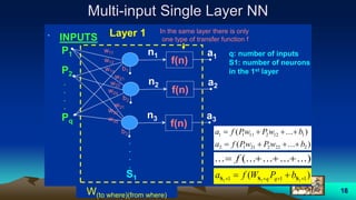
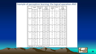
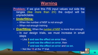
• In anfis we always have single output.
• If we have (MISO) , Example
– Inputs are X, Y which are two vectors 1*n
– Output is Z which is one vector 1*n
The training matrix will be
DataT=[X’ Y’ Z’] which is a matrix n*3