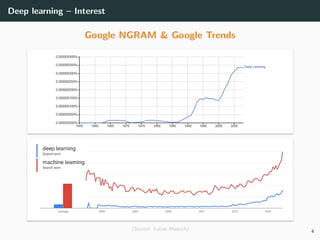
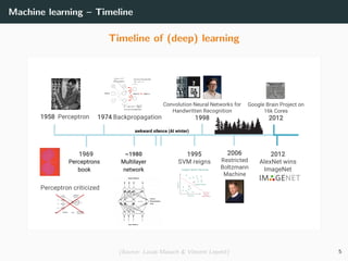
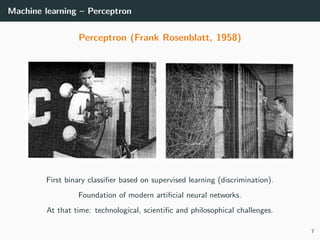
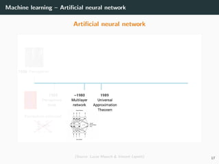
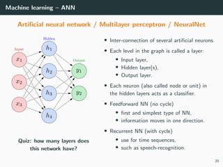
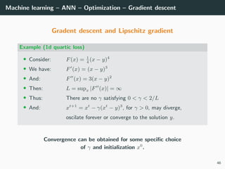
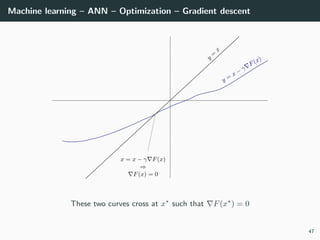
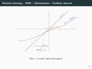
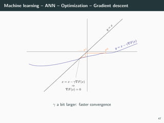
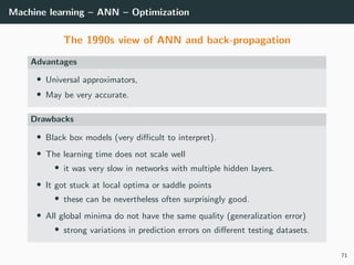
This document provides an overview of deep learning and its historical context within machine learning, detailing significant milestones from the inception of artificial neural networks to contemporary advancements. Key concepts such as the perceptron, training algorithms, and the importance of activation functions are discussed, highlighting their roles in the evolution of neural networks. The timeline traces the development of various techniques, emphasizing the resurgence of deep learning techniques in recent years.
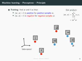
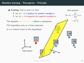
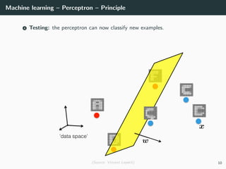
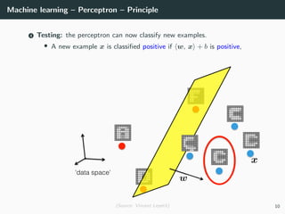
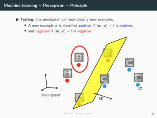
![Machine learning – ANN – Activation functions
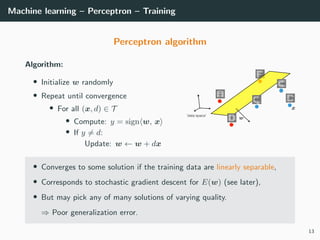
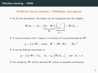
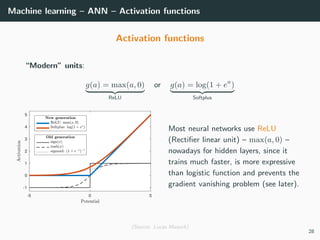
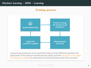
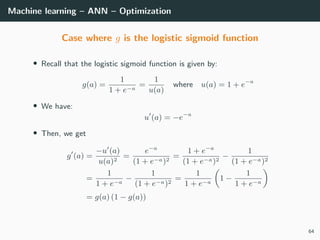
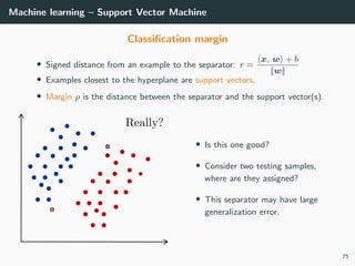
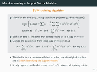
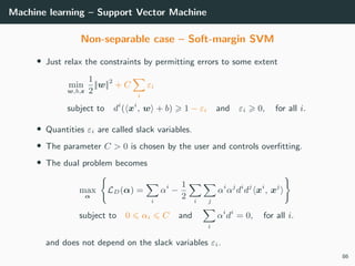
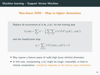
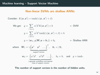
Activation functions
Sigmoidal units: for instance the hyperbolic tangent function
g(a) = tanh a =
ea
− e−a
ea + e−a
∈ [−1, 1]
or the logistic sigmoid function
g(a) =
1
1 + e−a
∈ [0, 1] -5 0 5
-2
-1
0
1
2
• In fact equivalent by linear transformations :
tanh(a/2) = 2logistic(a) − 1
• Differentiable approximations of the step and sign functions, respectively.
• Act as threshold units for large values of |a| and as linear for small values.
26](https://image.slidesharecdn.com/2predeep-190329010403/85/MLIP-Chapter-2-Preliminaries-to-deep-learning-35-320.jpg)
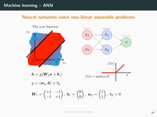
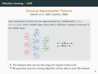
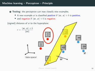
![Tasks, architectures and loss functions
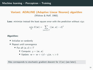
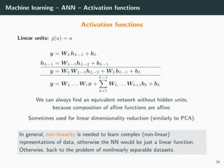
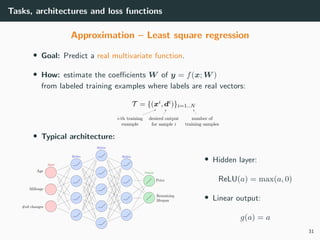
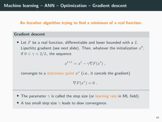
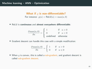
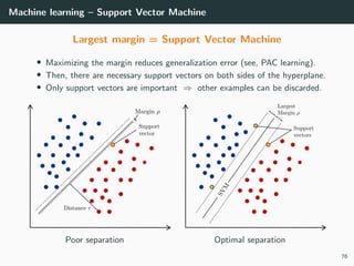
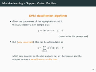
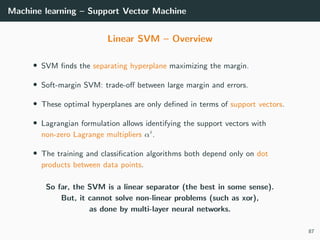
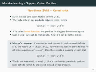
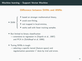
Approximation – Least square regression
• Loss: As for the polynomial curve fitting, it is standard to consider the
sum of square errors (assumption of Gaussian distributed errors)
E(W ) =
N
i=1
||yi
− di
||2
2 =
N
i=1
||f(xi
; W ) − di
||2
2
and look for W ∗
such that E(W ∗
) = 0. Recall: SSE ≡ SSD ≡ MSE
• Solution: Provided the network as enough flexibility and the size of the
training set grows to infinity
y = f(x; W ) = E[d|x] = dp(d|x) dd
posterior mean
32](https://image.slidesharecdn.com/2predeep-190329010403/85/MLIP-Chapter-2-Preliminaries-to-deep-learning-42-320.jpg)
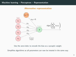
![Tasks, architectures and loss functions
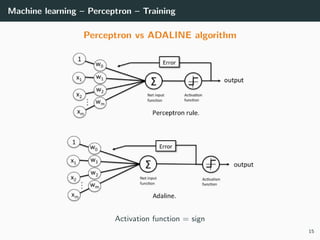
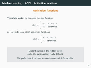
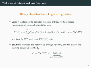
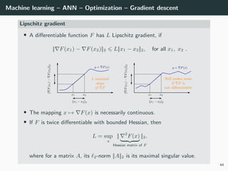
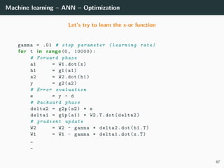
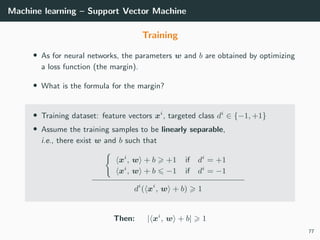
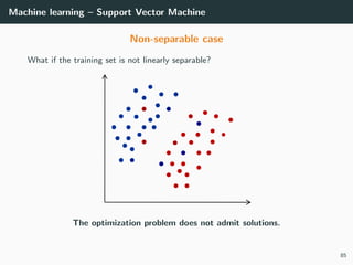
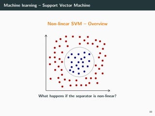
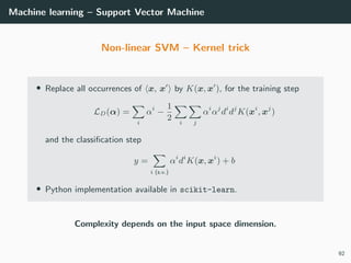
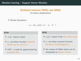
Binary classification – Logistic regression
• Goal: Classify object x into class C1 or C2.
• How: estimate the coefficients W of a real function y = f(x; W ) ∈ [0, 1]
from training examples with labels 1 (for class C1) and 0 (otherwise):
T = {(xi
, di
)}1=1..N
• Typical architecture:
• Hidden layer:
ReLU(a) = max(a, 0)
• Output layer:
logistic(x) =
1
1 + e−a
33](https://image.slidesharecdn.com/2predeep-190329010403/85/MLIP-Chapter-2-Preliminaries-to-deep-learning-43-320.jpg)
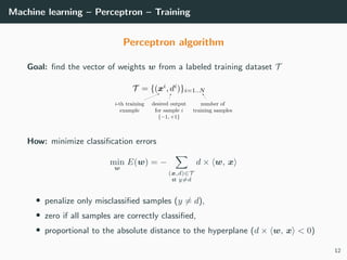
![Tasks, architectures and loss functions
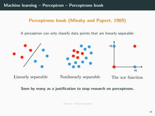
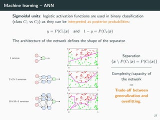
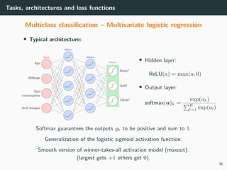
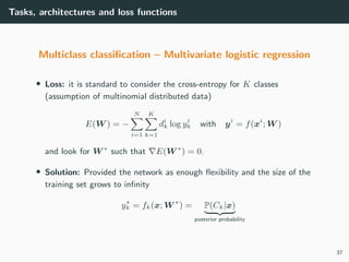
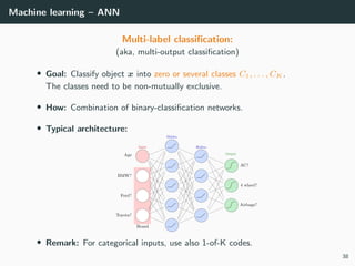
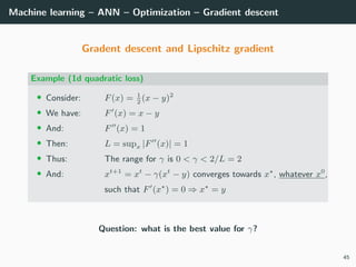
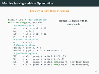
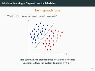
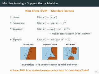
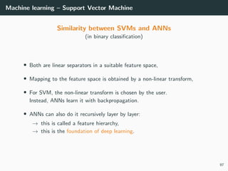
Multiclass classification – Multivariate logistic regression
(aka, multinomial classification)
• Goal: Classify an object x into one among K classes C1, . . . , CK .
• How: estimate the coefficients W of a multivariate function
y = f(x; W ) ∈ [0, 1]K
from training examples T = {(xi
, di
)} where di
is a 1-of-K (one-hot) code
• Class 1: di
= (1, 0, . . . , 0)T
if xi
∈ C1
• Class 2: di
= (0, 1, . . . , 0)T
if xi
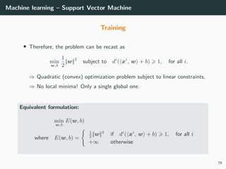
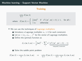
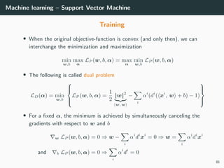
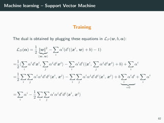
∈ C2
• . . .
• Class K: di
= (0, 0, . . . , 1)T
if xi
∈ CK
• Remark: do not use the class index k directly as a scalar label.
35](https://image.slidesharecdn.com/2predeep-190329010403/85/MLIP-Chapter-2-Preliminaries-to-deep-learning-45-320.jpg)
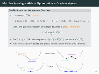
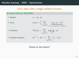
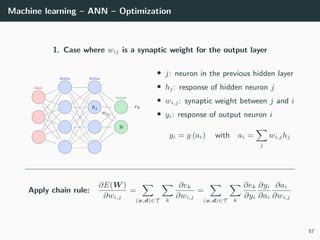
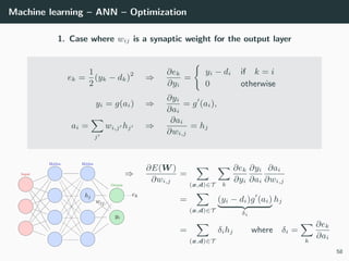
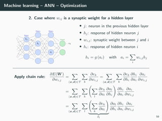
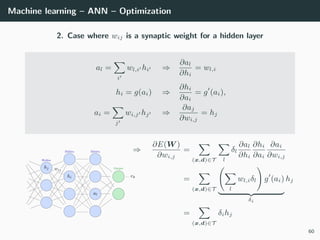
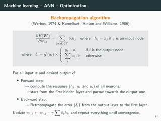
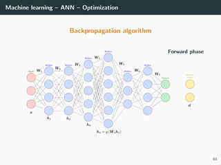
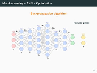
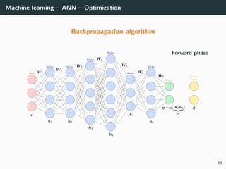
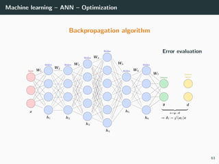
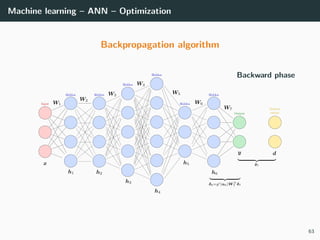
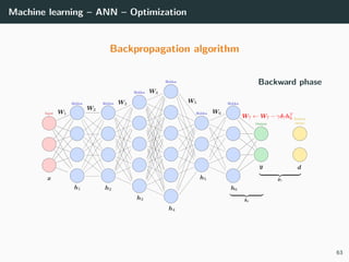
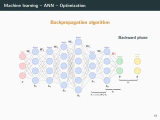
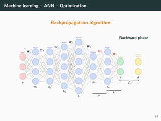
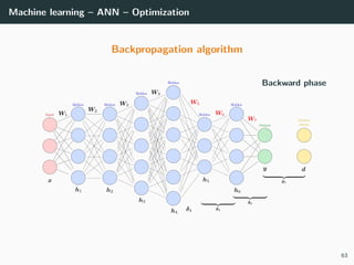
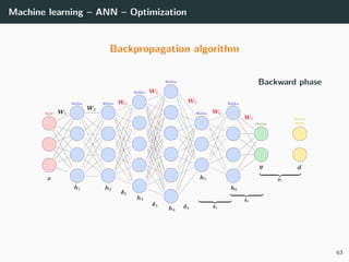
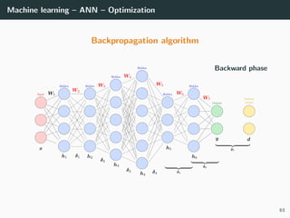
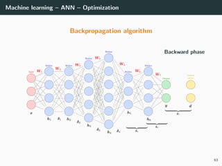
![Machine learning – ANN – Optimization
Objective: min
W
E(W ) ⇒ E(W ) = ∂E(W )
∂W1
. . . ∂E(W )
∂WL
T
= 0
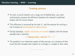
Loss functions: recall that classical loss functions are
• Square error (for regression: dk ∈ R, yk ∈ R)
E(W ) =
1
2
(x,d)∈T
||y − d||2
2 =
1
2
(x,d)∈T k
(yk − dk)2
• Cross-entropy (for multi-class classification: dk ∈ {0, 1}, yk ∈ [0, 1])
E(W ) = −
(x,d)∈T k
dk log yk
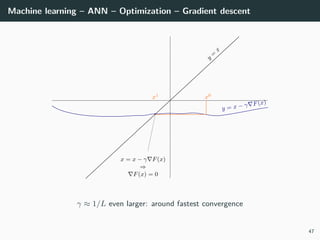
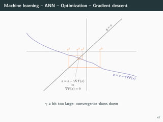
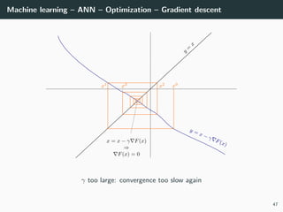
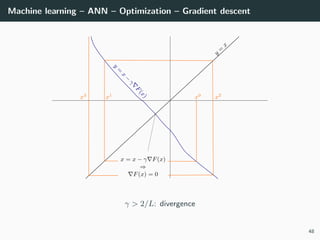
Solution: no close-form solutions ⇒ use gradient descent. What is it?
42](https://image.slidesharecdn.com/2predeep-190329010403/85/MLIP-Chapter-2-Preliminaries-to-deep-learning-53-320.jpg)
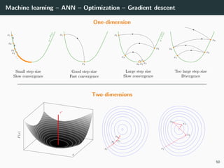
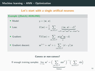
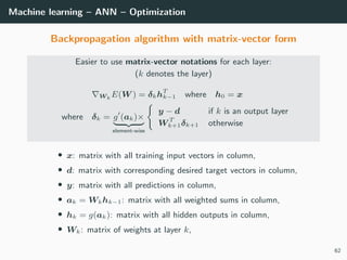
![Machine learning – ANN – Optimization
Back to our optimization problem
In our case W → E(W ) is non-convex ⇒ No guarantee of convergence.
Convergence will depends on
• the initialization,
• the step size γ.
Because of this:
• Normalizing each data point x in the range [−1, +1] is important to
control for the Hessian → the stability and the speed of the algorithm,
• The activation functions and the loss should be chosen to have a second
derivative smaller than 1 (when combined),
• The initialization should be random with well chosen variance
(we will go back to this later),
• If all of these are satisfied, we can generally choose γ ∈ [.001, 1].
54](https://image.slidesharecdn.com/2predeep-190329010403/85/MLIP-Chapter-2-Preliminaries-to-deep-learning-71-320.jpg)
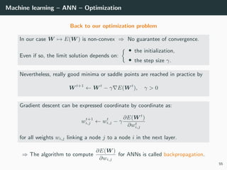

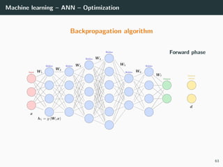


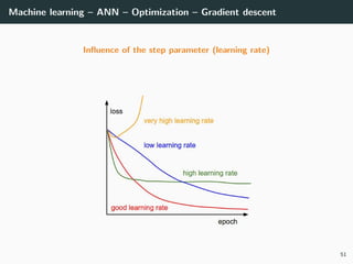
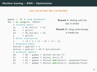
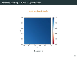
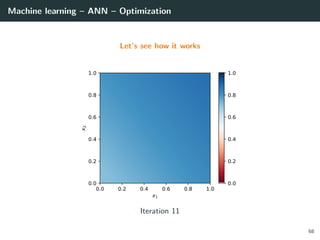
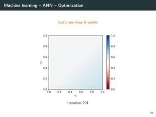
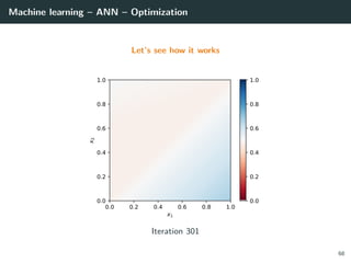
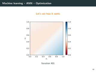
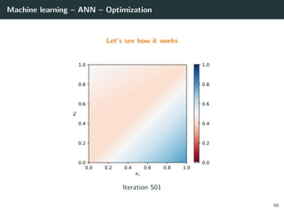
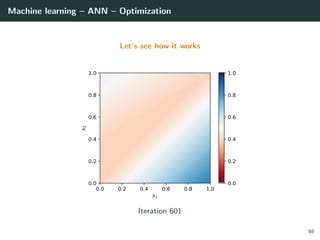
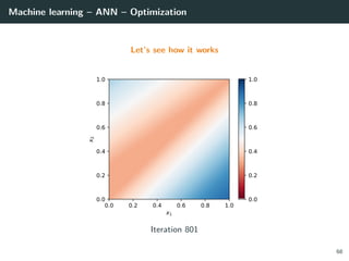
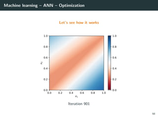
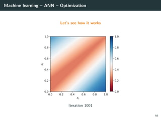
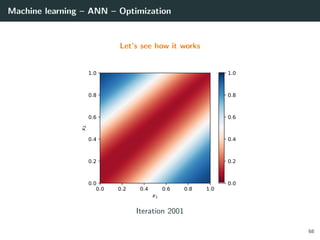
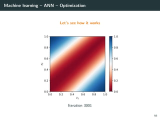
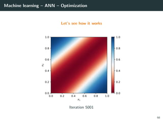
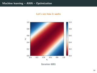
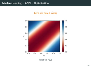
![Machine learning – ANN – Optimization
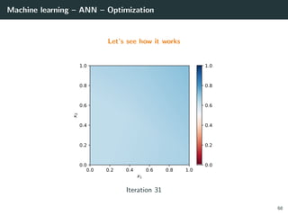
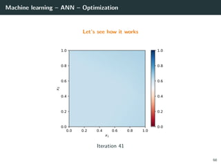
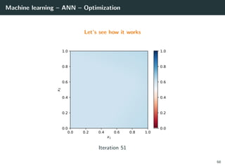
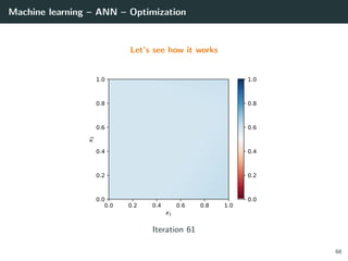
Let’s try to learn the x-or function
import numpy as np
# Training set
x = np.array ([[0 ,0] , [0,1], [1,0], [1 ,1]]).T
d = np.array ([ 0, +1, +1, 0 ]).T
# Initialization for a 2 layer feedforward network
b1 = np.random.rand(2, 1)
W1 = np.random.rand(2, 2)
b2 = np.random.rand(1, 1)
W2 = np.random.rand(1, 2)
# Activation functions and their derivatives
def g1(a): return a * (a > 0) # ReLU
def g1p(a): return 1 * (a > 0)
def g2(a): return a # Linear
def g2p(a): return 1
66](https://image.slidesharecdn.com/2predeep-190329010403/85/MLIP-Chapter-2-Preliminaries-to-deep-learning-100-320.jpg)
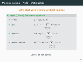
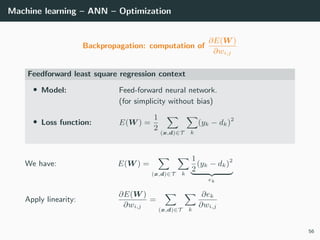
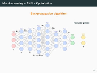
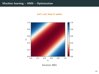
![Machine learning – ANN – Optimization
Let’s try to learn the x-or function
import numpy as np
# Training set
x = np.array ([[0 ,0] , [0,1], [1,0], [1 ,1]]).T
d = np.array ([ 0, +1, +1, 0 ]).T
# Initialization for a 2 layer feedforward network
b1 = np.random.rand(2, 1)
W1 = np.random.rand(2, 2)
b2 = np.random.rand(1, 1)
W2 = np.random.rand(1, 2)
# Activation functions and their derivatives
def g1(a): return a * (a > 0) # ReLU
def g1p(a): return 1 * (a > 0)
def g2(a): return 1 / (1 + np.exp(-a)) # Logistic
def g2p(a): return g2(a) * (1 - g2(a))
66](https://image.slidesharecdn.com/2predeep-190329010403/85/MLIP-Chapter-2-Preliminaries-to-deep-learning-101-320.jpg)


![[PR12] PR-036 Learning to Remember Rare Events](https://cdn.slidesharecdn.com/ss_thumbnails/pr12pr-036learningtoremeberrareevents-170917140144-thumbnail.jpg?width=640&height=640&fit=bounds)


![[Deck] What's New in Spark-Iceberg Integration via DSV2.pptx](https://cdn.slidesharecdn.com/ss_thumbnails/deckwhatsnewinspark-icebergintegrationviadsv2-260210005337-25955b12-thumbnail.jpg?width=640&height=640&fit=bounds)


