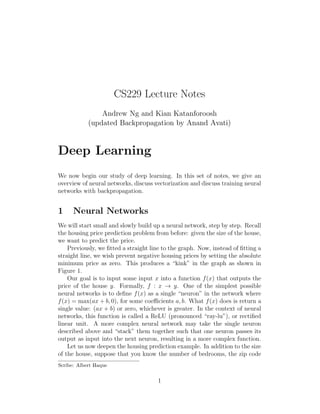
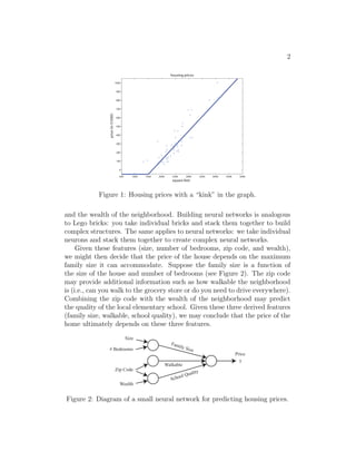
This summary provides an overview of the key points from the CS229 lecture notes document: 1. The document introduces neural networks and discusses representing simple neural networks as "stacks" of individual neuron units. It uses a housing price prediction example to illustrate this concept. 2. More complex neural networks can have multiple input features that are connected to hidden units, which may learn intermediate representations to predict the output. 3. Vectorization techniques are discussed to efficiently compute the outputs of all neurons in a layer simultaneously, without using slow for loops. Matrix operations allow representing the computations in a way that can leverage optimized linear algebra software.

1. CS229 Lecture Notes
Andrew Ng and Kian Katanforoosh
(updated Backpropagation by Anand Avati)
Deep Learning
We now begin our study of deep learning. In this set of notes, we give an
overview of neural networks, discuss vectorization and discuss training neural
networks with backpropagation.
1 Neural Networks
We will start small and slowly build up a neural network, step by step. Recall
the housing price prediction problem from before: given the size of the house,
we want to predict the price.
Previously, we fitted a straight line to the graph. Now, instead of fitting a
straight line, we wish prevent negative housing prices by setting the absolute
minimum price as zero. This produces a “kink” in the graph as shown in
Figure 1.
Our goal is to input some input x into a function f(x) that outputs the
price of the house y. Formally, f : x → y. One of the simplest possible
neural networks is to define f(x) as a single “neuron” in the network where
f(x) = max(ax + b, 0), for some coefficients a, b. What f(x) does is return a
single value: (ax + b) or zero, whichever is greater. In the context of neural
networks, this function is called a ReLU (pronounced “ray-lu”), or rectified
linear unit. A more complex neural network may take the single neuron
described above and “stack” them together such that one neuron passes its
output as input into the next neuron, resulting in a more complex function.
Let us now deepen the housing prediction example. In addition to the size
of the house, suppose that you know the number of bedrooms, the zip code
Scribe: Albert Haque
1

2. 2
500 1000 1500 2000 2500 3000 3500 4000 4500 5000
0
100
200
300
400
500
600
700
800
900
1000
housing prices
square feet
price(in$1000)
Figure 1: Housing prices with a “kink” in the graph.
and the wealth of the neighborhood. Building neural networks is analogous
to Lego bricks: you take individual bricks and stack them together to build
complex structures. The same applies to neural networks: we take individual
neurons and stack them together to create complex neural networks.
Given these features (size, number of bedrooms, zip code, and wealth),
we might then decide that the price of the house depends on the maximum
family size it can accommodate. Suppose the family size is a function of
the size of the house and number of bedrooms (see Figure 2). The zip code
may provide additional information such as how walkable the neighborhood
is (i.e., can you walk to the grocery store or do you need to drive everywhere).
Combining the zip code with the wealth of the neighborhood may predict
the quality of the local elementary school. Given these three derived features
(family size, walkable, school quality), we may conclude that the price of the
home ultimately depends on these three features.
Family Size
School Quality
Walkable
Size
# Bedrooms
Zip Code
Wealth
Price
y
Figure 2: Diagram of a small neural network for predicting housing prices.

3. 3
We have described this neural network as if you (the reader) already have
the insight to determine these three factors ultimately affect the housing
price. Part of the magic of a neural network is that all you need are the
input features x and the output y while the neural network will figure out
everything in the middle by itself. The process of a neural network learning
the intermediate features is called end-to-end learning.
Following the housing example, formally, the input to a neural network is
a set of input features x1, x2, x3, x4. We connect these four features to three
neurons. These three ”internal” neurons are called hidden units. The goal for
the neural network is to automatically determine three relevant features such
that the three features predict the price of a house. The only thing we must
provide to the neural network is a sufficient number of training examples
(x(i)
, y(i)
). Often times, the neural network will discover complex features
which are very useful for predicting the output but may be difficult for a
human to understand since it does not have a “common” meaning. This is
why some people refer to neural networks as a black box, as it can be difficult
to understand the features it has invented.
Let us formalize this neural network representation. Suppose we have
three input features x1, x2, x3 which are collectively called the input layer,
four hidden units which are collectively called the hidden layer and one out-
put neuron called the output layer. The term hidden layer is called “hidden”
because we do not have the ground truth/training value for the hidden units.
This is in contrast to the input and output layers, both of which we know
the ground truth values from (x(i)
, y(i)
).
The first hidden unit requires the input x1, x2, x3 and outputs a value
denoted by a1. We use the letter a since it refers to the neuron’s “activation”
value. In this particular example, we have a single hidden layer but it is
possible to have multiple hidden layers. Let a
[1]
1 denote the output value of
the first hidden unit in the first hidden layer. We use zero-indexing to refer
to the layer numbers. That is, the input layer is layer 0, the first hidden
layer is layer 1 and the output layer is layer 2. Again, more complex neural
networks may have more hidden layers. Given this mathematical notation,
the output of layer 2 is a
[2]
1 . We can unify our notation:
x1 = a
[0]
1 (1.1)
x2 = a
[0]
2 (1.2)
x3 = a
[0]
3 (1.3)
To clarify, foo[1]
with brackets denotes anything associated with layer 1, x(i)
with parenthesis refers to the ith
training example, and a
[ ]
j refers to the

4. 4
activation of the jth
unit in layer . If we look at logistic regression g(x) as
a single neuron (see Figure 3):
g(x) =
1
1 + exp(−wT x)
The input to the logistic regression g(x) is three features x1, x2 and x3 and it
outputs an estimated value of y. We can represent g(x) with a single neuron
in the neural network. We can break g(x) into two distinct computations:
(1) z = wT
x + b and (2) a = σ(z) where σ(z) = 1/(1 + e−z
). Note the
notational difference: previously we used z = θT
x but now we are using
z = wT
x+b, where w is a vector. Later in these notes you will see capital W
to denote a matrix. The reasoning for this notational difference is conform
with standard neural network notation. More generally, a = g(z) where g(z)
is some activation function. Example activation functions include:
g(z) =
1
1 + e−z
(sigmoid) (1.4)
g(z) = max(z, 0) (ReLU) (1.5)
g(z) =
ez
− e−z
ez + e−z
(tanh) (1.6)
In general, g(z) is a non-linear function.
x1
x2
x3
Estimated
value of y
Figure 3: Logistic regression as a single neuron.
Returning to our neural network from before, the first hidden unit in the first
hidden layer will perform the following computation:
z
[1]
1 = W
[1]
1
T
x + b
[1]
1 and a
[1]
1 = g(z
[1]
1 ) (1.7)
where W is a matrix of parameters and W1 refers to the first row of this
matrix. The parameters associated with the first hidden unit is the vector

5. 5
W
[1]
1 ∈ R3
and the scalar b
[1]
1 ∈ R. For the second and third hidden units in
the first hidden layer, the computation is defined as:
z
[1]
2 = W
[1]
2
T
x + b
[1]
2 and a
[1]
2 = g(z
[1]
2 )
z
[1]
3 = W
[1]
3
T
x + b
[1]
3 and a
[1]
3 = g(z
[1]
3 )
where each hidden unit has its corresponding parameters W and b. Moving
on, the output layer performs the computation:
z
[2]
1 = W
[2]
1
T
a[1]
+ b
[2]
1 and a
[2]
1 = g(z
[2]
1 ) (1.8)
where a[1]
is defined as the concatenation of all first layer activations:
a[1]
=





a
[1]
1
a
[1]
2
a
[1]
3
a
[1]
4





(1.9)
The activation a
[2]
1 from the second layer, which is a single scalar as defined by
a
[2]
1 = g(z
[2]
1 ), represents the neural network’s final output prediction. Note
that for regression tasks, one typically does not apply a non-linear function
which is strictly positive (i.e., ReLU or sigmoid) because for some tasks, the
ground truth y value may in fact be negative.
2 Vectorization
In order to implement a neural network at a reasonable speed, one must be
careful when using for loops. In order to compute the hidden unit activations
in the first layer, we must compute z1, ..., z4 and a1, ..., a4.
z
[1]
1 = W
[1]
1
T
x + b
[1]
1 and a
[1]
1 = g(z
[1]
1 ) (2.1)
...
...
... (2.2)
z
[1]
4 = W
[1]
4
T
x + b
[1]
4 and a
[1]
4 = g(z
[1]
4 ) (2.3)
The most natural way to implement this in code is to use a for loop. One of
the treasures that deep learning has given to the field of machine learning is
that deep learning algorithms have high computational requirements. As a
result, code will run very slowly if you use for loops.

6. 6
This gave rise to vectorization. Instead of using for loops, vectorization
takes advantage of matrix algebra and highly optimized numerical linear
algebra packages (e.g., BLAS) to make neural network computations run
quickly. Before the deep learning era, a for loop may have been sufficient
on smaller datasets, but modern deep networks and state-of-the-art datasets
will be infeasible to run with for loops.
2.1 Vectorizing the Output Computation
We now present a method for computing z1, ..., z4 without a for loop. Using
our matrix algebra, we can compute the activations:






z
[1]
1
...
...
z
[1]
4






z[1]
∈ R4×1
=






— W
[1]
1
T
—
— W
[1]
2
T
—
...
— W
[1]
4
T
—






W[1]
∈ R4×3


x1
x2
x3


x ∈ R3×1
+





b
[1]
1
b
[1]
2
...
b
[1]
4





b[1]
∈ R4×1
(2.4)
Where the Rd×n
beneath each matrix indicates the dimensions. Expressing
this in matrix notation: z[1]
= W[1]
x + b[1]
. To compute a[1]
without a
for loop, we can leverage vectorized libraries in Matlab, Octave, or Python
which compute a[1]
= g(z[1]
) very fast by performing parallel element-wise
operations. Mathematically, we defined the sigmoid function g(z) as:
g(z) =
1
1 + e−z
where z ∈ R (2.5)
However, the sigmoid function can be defined not only for scalars but also
vectors. In a Matlab/Octave-like pseudocode, we can define the sigmoid as:
g(z) = 1 ./ (1+exp(-z)) where z ∈ Rd
(2.6)
where ./ denotes element-wise division. With this vectorized implementa-
tion, a[1]
= g(z[1]
) can be computed quickly.
To summarize the neural network so far, given an input x ∈ R3
, we com-
pute the hidden layer’s activations with z[1]
= W[1]
x + b[1]
and a[1]
= g(z[1]
).
To compute the output layer’s activations (i.e., neural network output):
z[2]
1×1
= W[2]
1×4
a[1]
4×1
+ b[2]
1×1
and a[2]
1×1
= g( z[2]
1×1
) (2.7)

7. 7
Why do we not use the identity function for g(z)? That is, why not use
g(z) = z? Assume for sake of argument that b[1]
and b[2]
are zeros. Using
Equation (2.7), we have:
z[2]
= W[2]
a[1]
(2.8)
= W[2]
g(z[1]
) by definition (2.9)
= W[2]
z[1]
since g(z) = z (2.10)
= W[2]
W[1]
x from Equation (2.4) (2.11)
= ˜Wx where ˜W = W[2]
W[1]
(2.12)
Notice how W[2]
W[1]
collapsed into ˜W. This is because applying a linear
function to another linear function will result in a linear function over the
original input (i.e., you can construct a ˜W such that ˜Wx = W[2]
W[1]
x).
This loses much of the representational power of the neural network as often
times the output we are trying to predict has a non-linear relationship with
the inputs. Without non-linear activation functions, the neural network will
simply perform linear regression.
2.2 Vectorization Over Training Examples
Suppose you have a training set with three examples. The activations for
each example are as follows:
z[1](1)
= W[1]
x(1)
+ b[1]
z[1](2)
= W[1]
x(2)
+ b[1]
z[1](3)
= W[1]
x(3)
+ b[1]
Note the difference between square brackets [·], which refer to the layer num-
ber, and parenthesis (·), which refer to the training example number. In-
tuitively, one would implement this using a for loop. It turns out, we can
vectorize these operations as well. First, define:
X =


| | |
x(1)
x(2)
x(3)
| | |

 (2.13)
Note that we are stacking training examples in columns and not rows. We
can then combine this into a single unified formulation:
Z[1]
=


| | |
z[1](1)
z[1](2)
z[1](3)
| | |

 = W[1]
X + b[1]
(2.14)

8. 8
You may notice that we are attempting to add b[1]
∈ R4×1
to W[1]
X ∈
R4×3
. Strictly following the rules of linear algebra, this is not allowed. In
practice however, this addition is performed using broadcasting. We create
an intermediate ˜b[1]
∈ R4×3
:
˜b[1]
=


| | |
b[1]
b[1]
b[1]
| | |

 (2.15)
We can then perform the computation: Z[1]
= W[1]
X + ˜b[1]
. Often times, it
is not necessary to explicitly construct ˜b[1]
. By inspecting the dimensions in
(2.14), you can assume b[1]
∈ R4×1
is correctly broadcast to W[1]
X ∈ R4×3
.
Putting it together: Suppose we have a training set (x(1)
, y(1)
), ..., (x(n)
, y(n)
)
where x(i)
is a picture and y(i)
is a binary label for whether the picture con-
tains a cat or not (i.e., 1=contains a cat). First, we initialize the parameters
W[1]
, b[1]
, W[2]
, b[2]
to small random numbers. For each example, we compute
the output “probability” from the sigmoid function a[2](i)
. Second, using the
logistic regression log likelihood:
n
i=1
y(i)
log a[2](i)
+ (1 − y(i)
) log(1 − a[2](i)
) (2.16)
Finally, we maximize this function using gradient ascent. This maximization
procedure corresponds to training the neural network.
3 Backpropagation
Instead of the housing example, we now have a new problem. Suppose we
wish to detect whether there is a soccer ball in an image or not. Given an
input image x(i)
, we wish to output a binary prediction 1 if there is a ball in
the image and 0 otherwise.
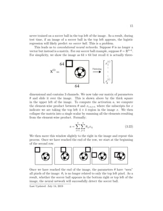
Aside: Images can be represented as a matrix with number of elements
equal to the number of pixels. However, color images are digitally represented
as a volume (i.e., three-channels; or three matrices stacked on each other).
The number three is used because colors are represented as red-green-blue
(RGB) values. In the diagram below, we have a 64×64×3 image containing
a soccer ball. It is flattened into a single vector containing 12,288 elements.
A neural network model consists of two components: (i) the network
architecture, which defines how many layers, how many neurons, and how
the neurons are connected and (ii) the parameters (values; also known as

9. 9
weights). In this section, we will talk about how to learn the parameters.
First we will talk about parameter initialization, optimization and analyzing
these parameters.
3.1 Parameter Initialization
Consider a two layer neural network. On the left, the input is a flattened
image vector x(1)
, ..., x
(i)
d . In the first hidden layer, notice how all inputs are
connected to all neurons in the next layer. This is called a fully connected
layer.
The next step is to compute how many parameters are in this network. One
way of doing this is to compute the forward propagation by hand.
z[1]
= W[1]
x(i)
+ b[1]
(3.1)
a[1]
= g(z[1]
) (3.2)
z[2]
= W[2]
a[1]
+ b[2]
(3.3)
a[2]
= g(z[2]
) (3.4)
z[3]
= W[3]
a[2]
+ b[3]
(3.5)
ˆy(i)
= a[3]
= g(z[3]
) (3.6)
We know that z[1]
, a[1]
∈ R3×1
and z[2]
, a[2]
∈ R2×1
and z[3]
, a[3]
∈ R1×1
. As
of now, we do not know the size of W[1]
. However, we can compute its size.

10. 10
We know that x ∈ Rd×1
. This leads us to the following
z[1]
= W[1]
x(i)
= R3×1
Written as sizes: R3×1
= R?×?
× Rd×1
(3.7)
Using matrix multiplication, we conclude that ?×? must be 3 × d. We also
conclude that the bias is of size 3 × 1 because its size must match W[1]
x(i)
.
We repeat this process for each hidden layer. This gives us:
W[2]
∈ R2×3
, b[2]
∈ R2×1
and W[3]
∈ R1×2
, b[3]
∈ R1×1
(3.8)
In total, we have 3n + 3 in the first layer, 2 × 3 + 2 in the second layer and
2 + 1 in the third layer. This gives us a total of 3n + 14 parameters.
Before we start training the neural network, we must select an initial
value for these parameters. We do not use the value zero as the initial value.
This is because the output of the first layer will always be the same since
W[1]
x(i)
+ b[1]
= 03×1
x(i)
+ 03×1
where 0d×n
denotes a matrix of size n × m
filled with zeros. This will cause problems later on when we try to update
these parameters (i.e., the gradients will all be the same). The solution is to
randomly initialize the parameters to small values (e.g., normally distributed
around zero; N(0, 0.1)). Once the parameters have been initialized, we can
begin training the neural network with gradient descent.
The next step of the training process is to update the parameters. After a
single forward pass through the neural network, the output will be a predicted
value ˆy. We can then compute the loss L, in our case the log loss:
L(ˆy, y) = − (1 − y) log(1 − ˆy) + y log ˆy (3.9)
The loss function L(ˆy, y) produces a single scalar value. For short, we will
refer to the loss value as L. Given this value, we now must update all
parameters in layers of the neural network. For any given layer index , we
update them:
W[ ]
= W[ ]
− α
∂L
∂W[ ]
(3.10)
b[ ]
= b[ ]
− α
∂L
∂b[ ]
(3.11)
where α is the learning rate. To proceed, we must compute the gradient with
respect to the parameters: ∂L/∂W[ ]
and ∂L/∂b[ ]
.
Remember, we made a decision to not set all parameters to zero. What if
we had initialized all parameters to be zero? We know that z[3]
= W[3]
a[2]
+b[3]

11. 11
will evaluate to zero, because W[3]
and b[3]
are all zero. However, the output
of the neural network is defined as a[3]
= g(z[3]
). Recall that g(·) is defined as
the sigmoid function. This means a[3]
= g(0) = 0.5. Thus, no matter what
value of x(i)
we provide, the network will output ˆy = 0.5.
What if we had initialized all parameters to be the same non-zero value?
In this case, consider the activations of the first layer:
a[1]
= g(z[1]
) = g(W[1]
x(i)
+ b[1]
) (3.12)
Each element of the activation vector a[1]
will be the same (because W[1]
contains all the same values). This behavior will occur at all layers of the
neural network. As a result, when we compute the gradient, all neurons in
a layer will be equally responsible for anything contributed to the final loss.
We call this property symmetry. This means each neuron (within a layer)
will receive the exact same gradient update value (i.e., all neurons will learn
the same thing).
In practice, it turns out there is something better than random initializa-
tion. It is called Xavier/He initialization and initializes the weights:
w[ ]
∼ N 0,
2
n[ ] + n[ −1]
(3.13)
where n[ ]
is the number of neurons in layer . This acts as a mini-normalization
technique. For a single layer, consider the variance of the input to the layer
as σ(in)
and the variance of the output (i.e., activations) of a layer to be
σ(out)
. Xavier/He initialization encourages σ(in)
to be similar to σ(out)
.
3.2 Optimization
Recall our neural network parameters: W[1]
, b[1]
, W[2]
, b[2]
, W[3]
, b[3]
. To up-
date them, we use stochastic gradient descent (SGD) using the update rules
in Equations (3.10) and (3.11). So our goal is to calculate ∂L
∂W[1] , ∂L
∂W[2] , ∂L
∂W[3] ,
∂L
∂b[1] , ∂L
∂b[2] and ∂L
∂b[3] . In what follows we will compute the gradient with respect
to W[2]
and leave the rest as an exercise since they are very similar.
First, observe that
∂L
∂W[2]
=
∂L
∂W
[2]
11
∂L
∂W
[2]
12
∂L
∂W
[2]
13
∂L
∂W
[2]
21
∂L
∂W
[2]
22
∂L
∂W
[2]
23
,
and also observe that
∂L
∂z[3]
=
∂
∂z[3]
[−y log ˆy − (1 − y) log(1 − ˆy)]

12. 12
=
∂
∂z[3]
−y log σ(z[3]
) − (1 − y) log(1 − σ(z[3]
)) (where σ is the sigmoid function)
= −y
1
σ(z[3])
σ(z[3]
)(1 − σ(z[3]
)) − (1 − y)
1
(1 − σ(z[3]))
(−1)σ(z[3]
)(1 − σ(z[3]
))
= −y(1 − σ(z[3]
) + (1 − y)σ(z[3]
)
= σ(z[3]
) − y
= a[3]
− y.
Now to calculate the gradient w.r.t ∂L
∂W
[2]
ij
, we use the multivariate chain
rule of calculus:
∂L
∂W
[2]
ij
=
∂L
∂ˆy
∂ˆy
∂W
[2]
ij
=
∂L
∂a[3]
∂a[3]
∂W
[2]
ij
=
∂L
∂a[3]
∂a[3]
∂z[3]
∂z[3]
∂W
[2]
ij
=
∂L
∂a[3]
∂a[3]
∂z[3]
∂z[3]
∂a[2]
∂a[2]
∂W
[2]
ij
=
∂L
∂a[3]
∂a[3]
∂z[3]
(a[3]
− y)
1×1
∂z[3]
∂a[2]
W[3]
1×2
∂a[2]
∂z[2]
diag g (z[2]
)
2×2
∂z[2]
∂W
[2]
ij
a
[1]
j ei
2×1
(where a[1]
∈ R3
, and ei ∈ R2
is the ith
basis vector)
= (a[3]
− y)W[3]
◦ g (z[2]
)
1×2
a
[1]
j ei
2×1
= (a[3]
− y)W[3]
◦ g (z[2]
) i
a
[1]
j
1×1
⇒
∂L
∂W[2]
= (a[3]
− y)W[3]
◦ g (z[2]
) a[1]T
2×3
where ◦ indicates elemntwise product (Hadamard product). We leave the
remaining gradients as an exercise to the reader.

13. 13
Returning to optimization, we previously discussed stochastic gradient
descent. Now we will talk about gradient descent. For any single layer , the
update rule is defined as:
W[ ]
= W[ ]
− α
∂J
∂W[ ]
(3.14)
where J is the cost function J = 1
n
n
i=1
L(i)
and L(i)
is the loss for a single exam-
ple. The difference between the gradient descent update versus the stochastic
gradient descent version is that the cost function J gives more accurate gra-
dients whereas L(i)
may be noisy. Stochastic gradient descent attempts to
approximate the gradient from (full) gradient descent. The disadvantage of
gradient descent is that it can be difficult to compute all activations for all
examples in a single forward or backwards propagation phase.
In practice, research and applications use mini-batch gradient descent.
This is a compromise between gradient descent and stochastic gradient de-
scent. In the case mini-batch gradient descent, the cost function Jmb is
defined as follows:
Jmb =
1
B
B
i=1
L(i)
(3.15)
where B is the number of examples in the mini-batch.
There is another optimization method called momentum. Consider mini-
batch stochastic gradient. For any single layer , the update rule is as follows:
vdW[ ] = βvdW[ ] + (1 − β) ∂J
∂W[ ]
W[ ]
= W[ ]
− αvdW[ ]
(3.16)
Notice how there are now two stages instead of a single stage. The weight
update now depends on the cost J at this update step and the velocity vdW[ ] .
The relative importance is controlled by β. Consider the analogy to a human
driving a car. While in motion, the car has momentum. If the car were to use
the brakes (or not push accelerator throttle), the car would continue moving
due to its momentum. Returning to optimization, the velocity vdW[ ] will
keep track of the gradient over time. This technique has significantly helped
neural networks during the training phase.
3.3 Analyzing the Parameters
At this point, we have initialized the parameters and have optimized the
parameters. Suppose we evaluate the trained model and observe that it

14. 14
achieves 96% accuracy on the training set but only 64% on the testing set.
Some solutions include: collecting more data, employing regularization, or
making the model shallower. Let us briefly look at regularization techniques.
3.3.1 L2 Regularization
Let W below denote all the parameters in a model. In the case of neural
networks, you may think of applying the 2nd term to all layer weights W[ ]
.
For convenience, we simply write W. The L2 regularization adds another
term to the cost function:
JL2 = J +
λ
2
||W||2
(3.17)
= J +
λ
2 ij
|Wij|2
(3.18)
= J +
λ
2
WT
W (3.19)
where J is the standard cost function from before, λ is an arbitrary value with
a larger value indicating more regularization and W contains all the weight
matrices, and where Equations (3.17), (3.18) and (3.19) are equivalent. The
update rule with L2 regularization becomes:
W = W − α
∂J
∂W
− α
λ
2
∂WT
W
∂W
(3.20)
= (1 − αλ)W − α
∂J
∂W
(3.21)
When we were updating our parameters using gradient descent, we did not
have the (1 − αλ)W term. This means with L2 regularization, every update
will include some penalization, depending on W. This penalization increases
the cost J, which encourages individual parameters to be small in magnitude,
which is a way to reduce overfitting.
3.3.2 Parameter Sharing
Recall logistic regression. It can be represented as a neural network, as
shown in Figure 3. The parameter vector θ = (θ1, ..., θd) must have the same
number of elements as the input vector x = (x1, ..., xd). In our image soccer
ball example, this means θ1 always looks at the top left pixel of the image
no matter what. However, we know that a soccer ball might appear in any
region of the image and not always the center. It is possible that θ1 was

15. 15
never trained on a soccer ball in the top left of the image. As a result, during
test time, if an image of a soccer ball in the top left appears, the logistic
regression will likely predict no soccer ball. This is a problem.
This leads us to convolutional neural networks. Suppose θ is no longer a
vector but instead is a matrix. For our soccer ball example, suppose θ = R4×4
.
For simplicity, we show the image as 64 × 64 but recall it is actually three-
dimensional and contains 3 channels. We now take our matrix of parameters
θ and slide it over the image. This is shown above by the thick square
in the upper left of the image. To compute the activation a, we compute
the element-wise product between θ and x1:4,1:4, where the subscripts for x
indicate we are taking the top left 4 × 4 region in the image x. We then
collapse the matrix into a single scalar by summing all the elements resulting
from the element-wise product. Formally:
a =
4
i=1
4
j=1
θijxij (3.22)
We then move this window slightly to the right in the image and repeat this
process. Once we have reached the end of the row, we start at the beginning
of the second row.
Once we have reached the end of the image, the parameters θ have “seen”
all pixels of the image: θ1 is no longer related to only the top left pixel. As a
result, whether the soccer ball appears in the bottom right or top left of the
image, the neural network will successfully detect the soccer ball.
Last Updated: July 14, 2019