Downloaded 161 times
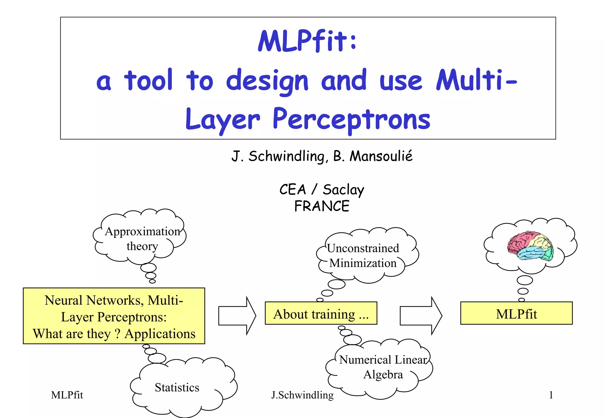

![2 theorems any continuous function (1 variable or more) on a compact set can be approximated to any accuracy by a linear combination of sigmoïds -> function approximation [ for example: K.Hornik et al. Multilayer Feedforward Networks are Universal Approximators , Neural Networks, Vol. 2, pp 359-366 (1989) ] trained with f(x) = 1 for signal and = 0 for background, the NN function approximates the probability of signal knowing x -> classification (cf Neyman-Pearson test) [for example: D.W.Ruck et al. The Multilayer Perceptron as an Approximation to a Bayes Optimal Discriminant Function , IEEE Transactions on Neural Networks, Vol. 1, n r 4, pp 296-298 (1990) ]](https://image.slidesharecdn.com/mlptool-090922010454-phpapp01/75/Multi-Layer-Perceptrons-5-2048.jpg)

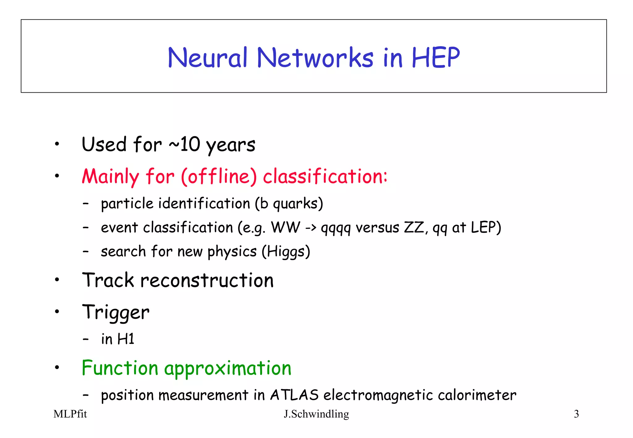
![Learning methods Stochastic minimization Linear model fixed steps [variable steps] Remarks: - derivatives known - other methods exist Global minimization Non-Linear weights All weights Linear model steepest descent with fixed steps or line search Quadratic model (Newton like) Conjugate gradients or BFGS with line search Solve LLS](https://image.slidesharecdn.com/mlptool-090922010454-phpapp01/75/Multi-Layer-Perceptrons-8-2048.jpg)
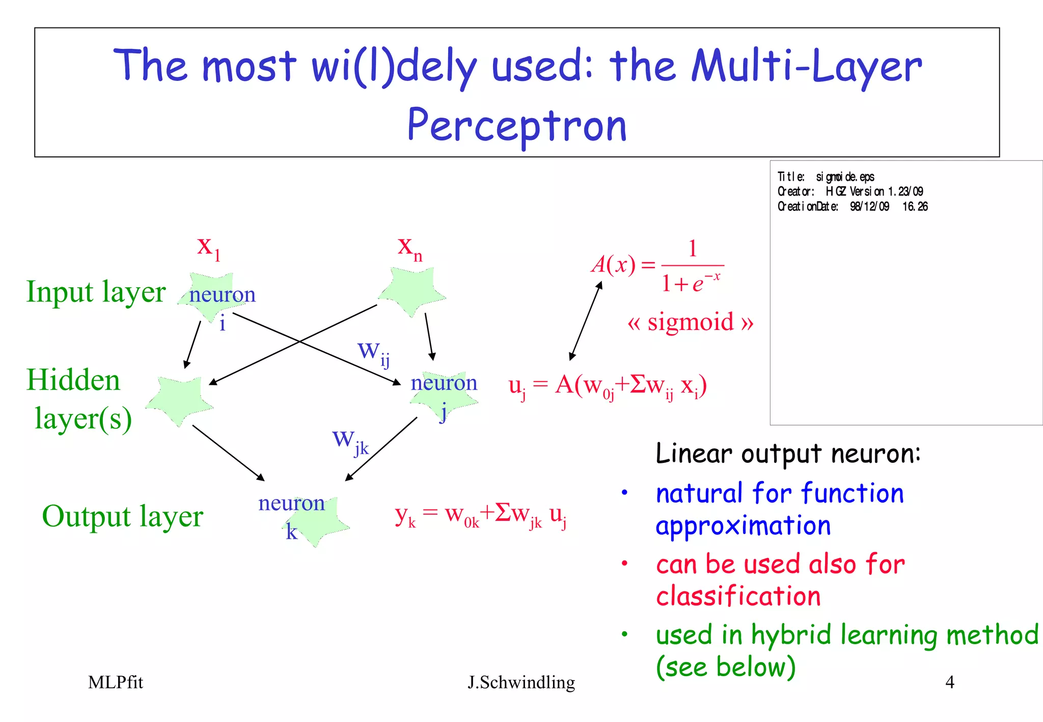
![Using MLPfit as a standalone package Reads ASCII files containing description of network, learning, running conditions examples (learn and test) [initial weights] Writes ASCII files containing output weights MLP (fortran or C) function Writes PAW file containing learning curves (Tested on HP-UX and alphavax / OSF) MLP_gen.c MLP_main.c PAWLIB MLP_lapack.c](https://image.slidesharecdn.com/mlptool-090922010454-phpapp01/75/Multi-Layer-Perceptrons-18-2048.jpg)
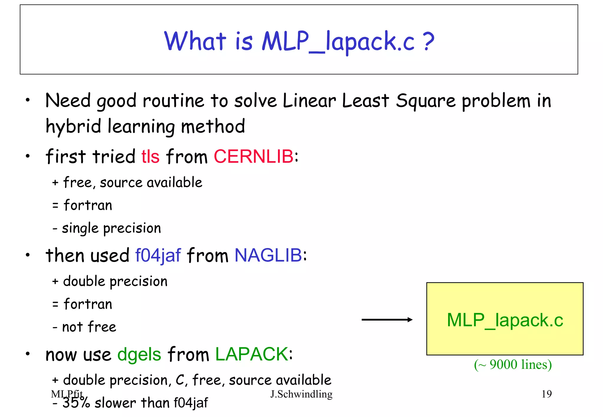
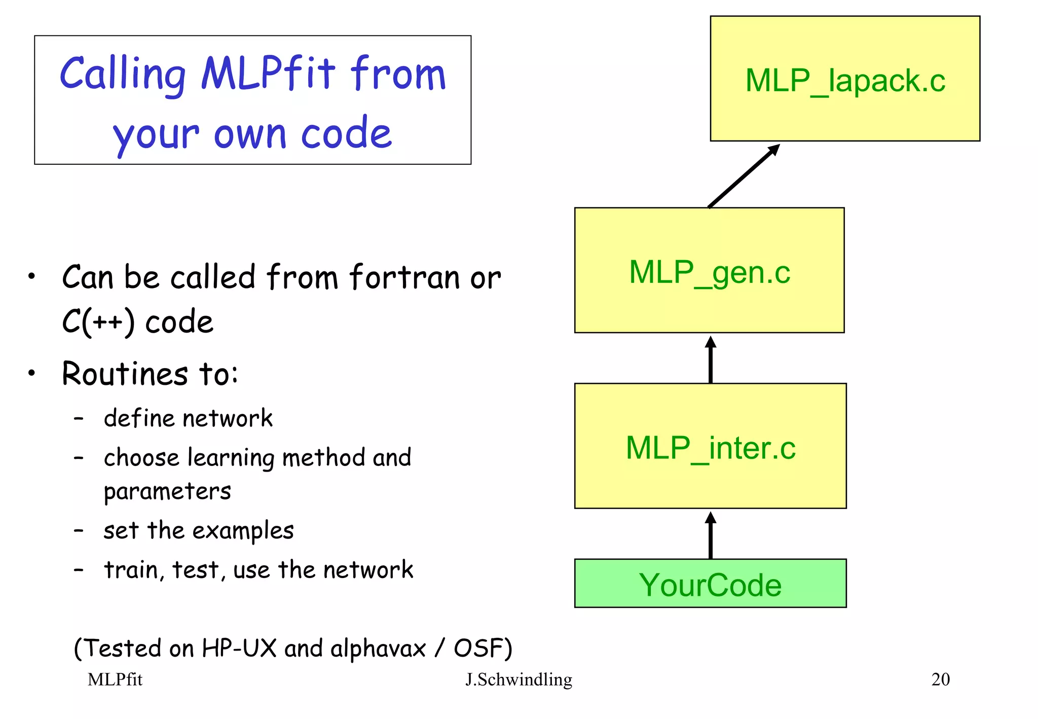
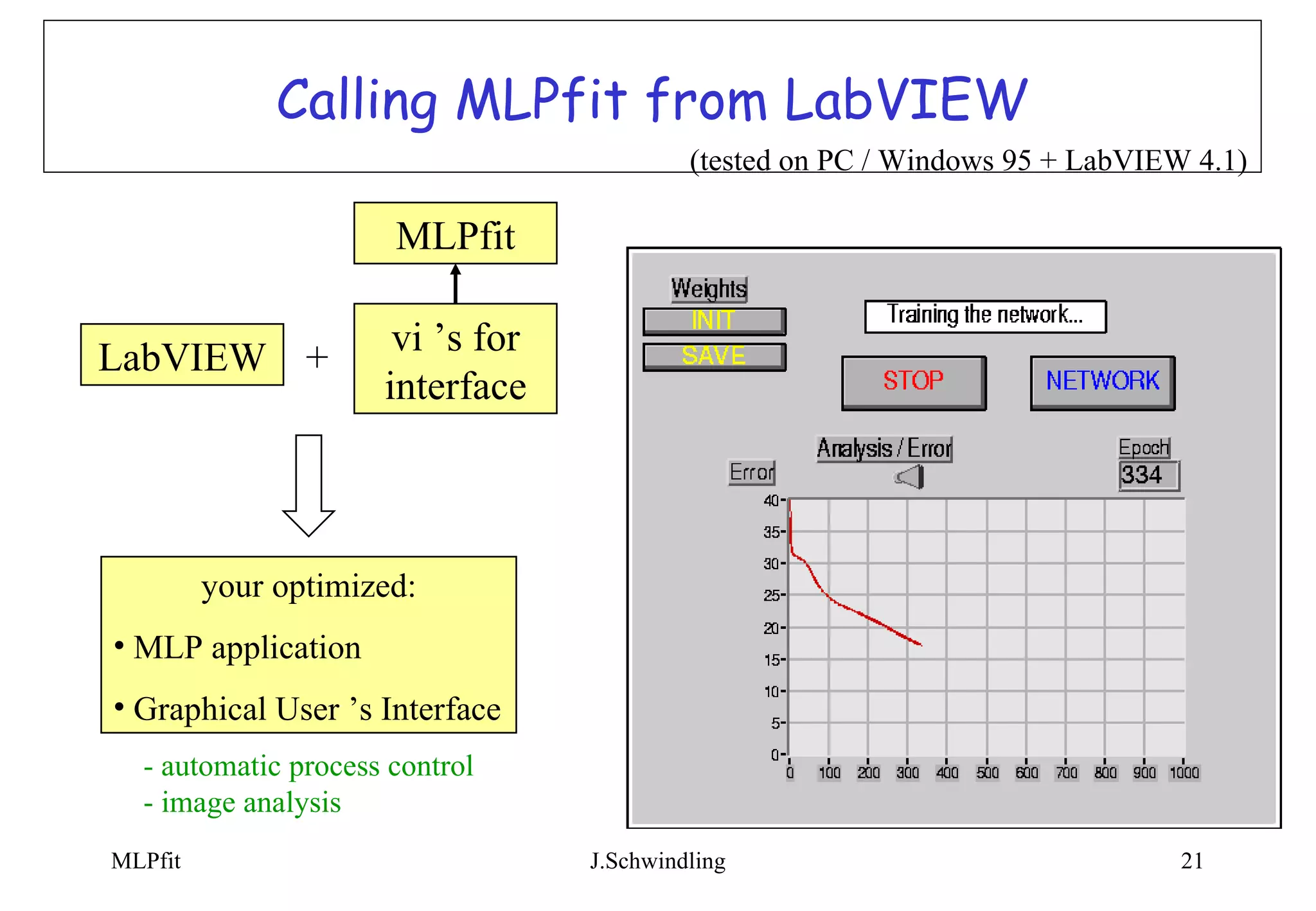
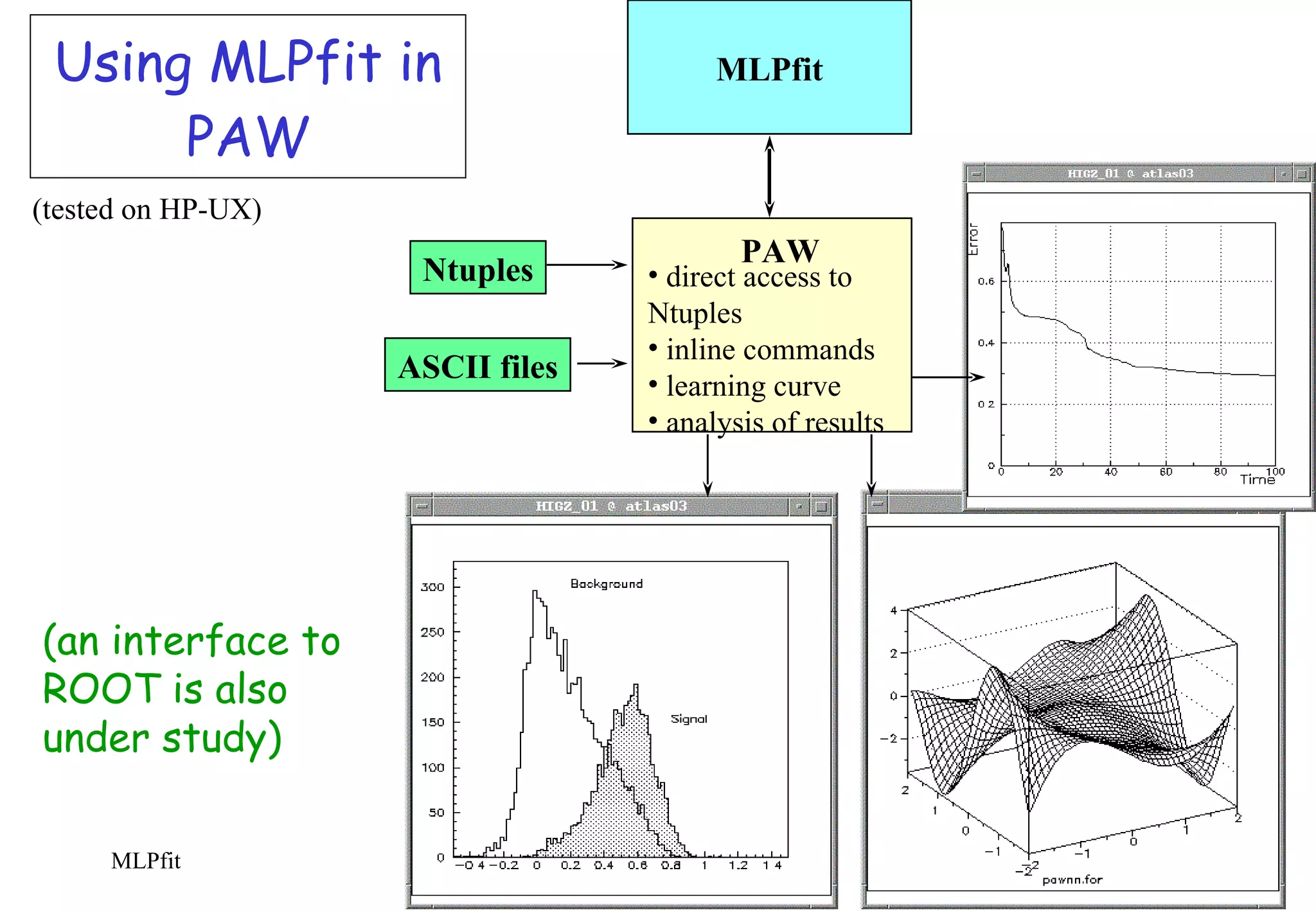
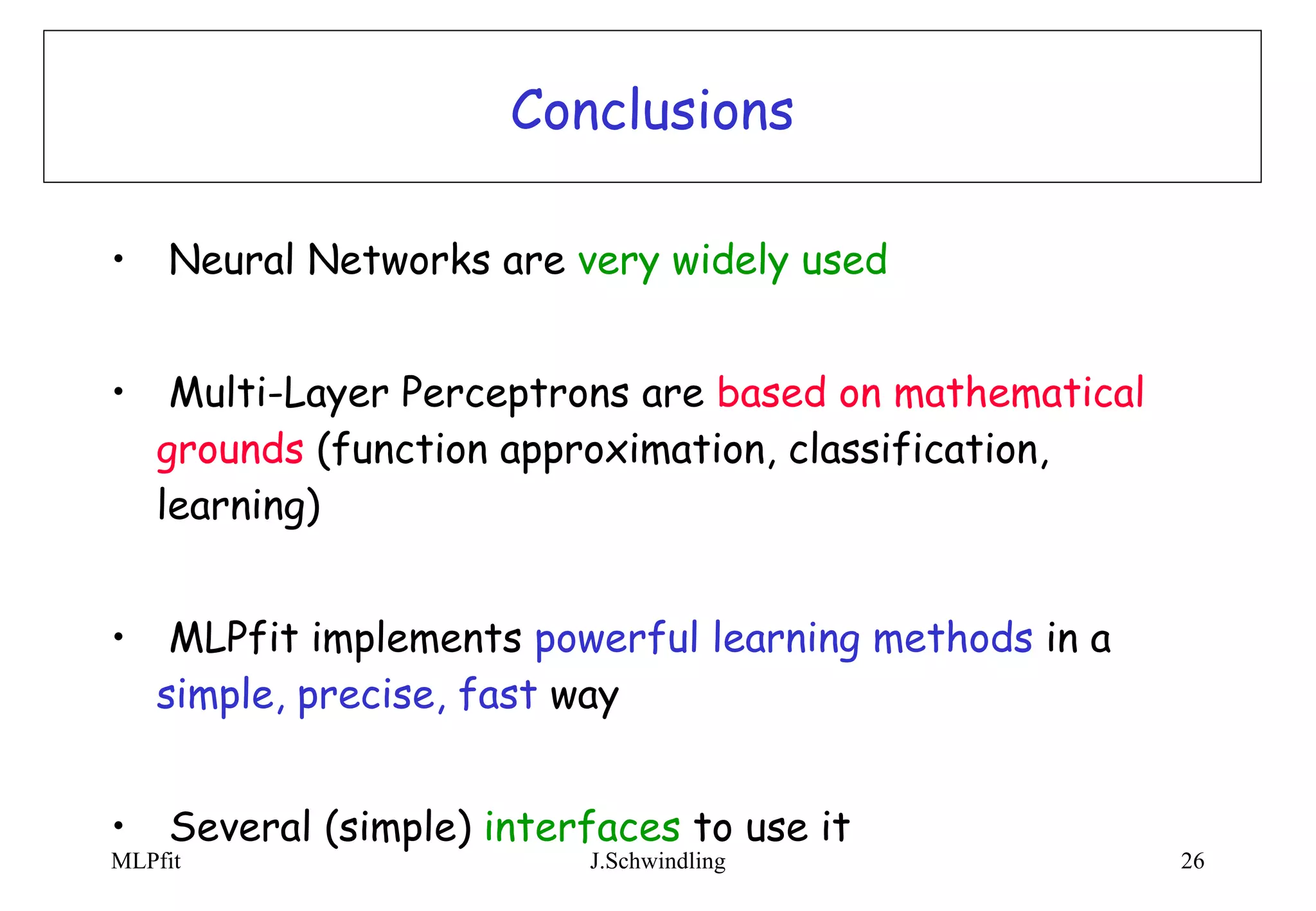

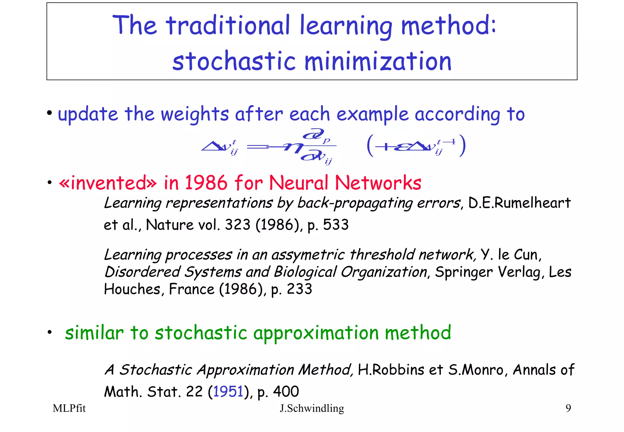
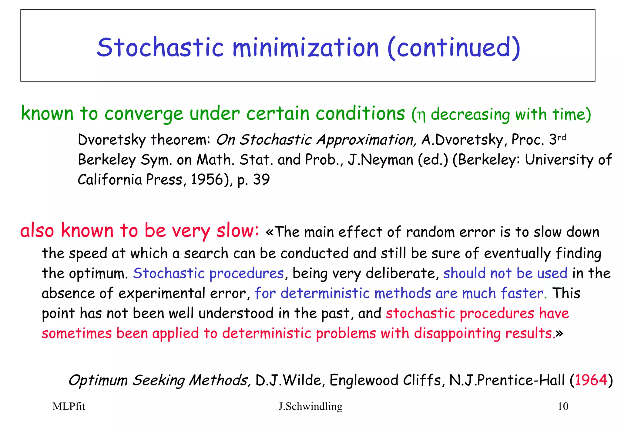
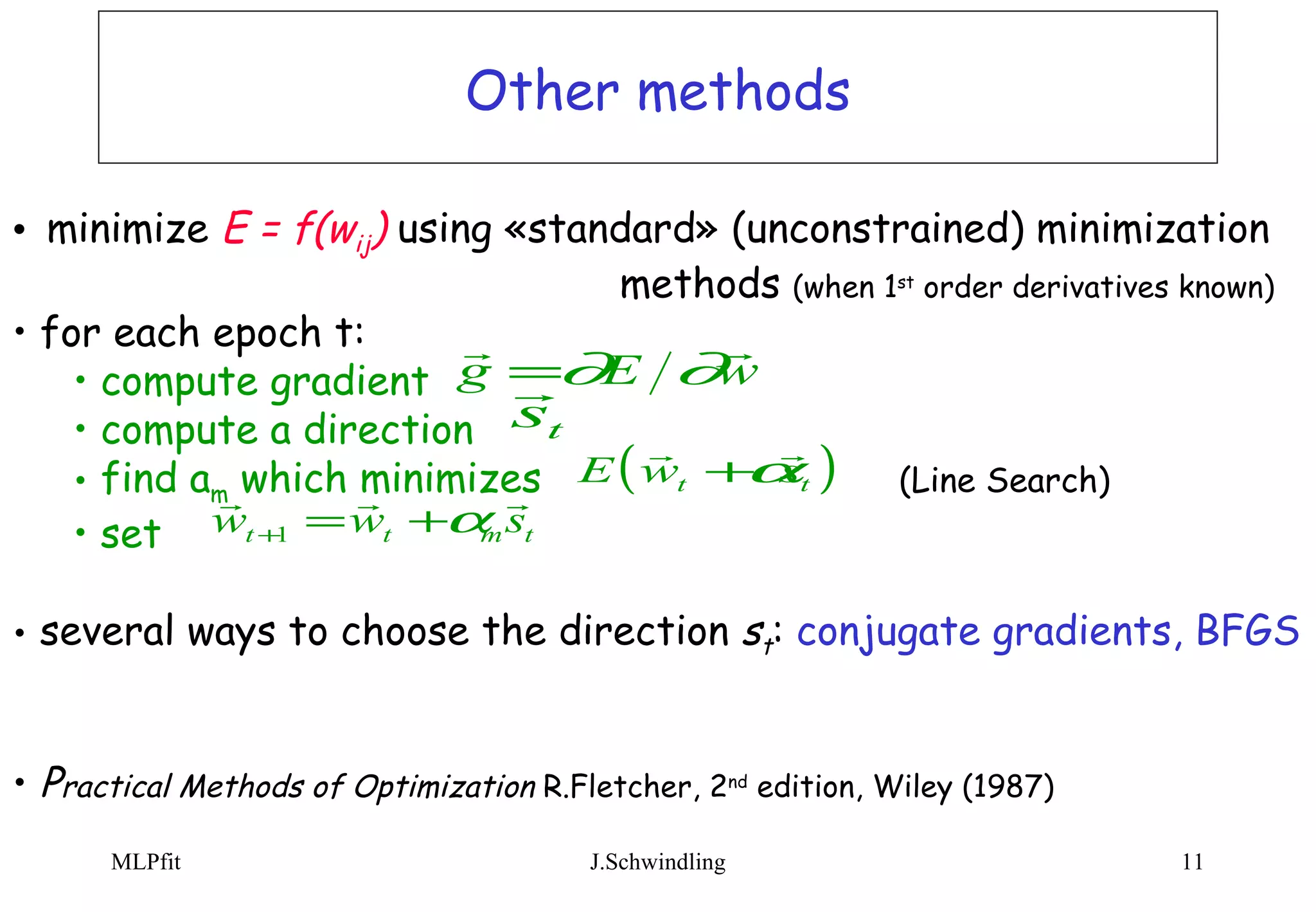
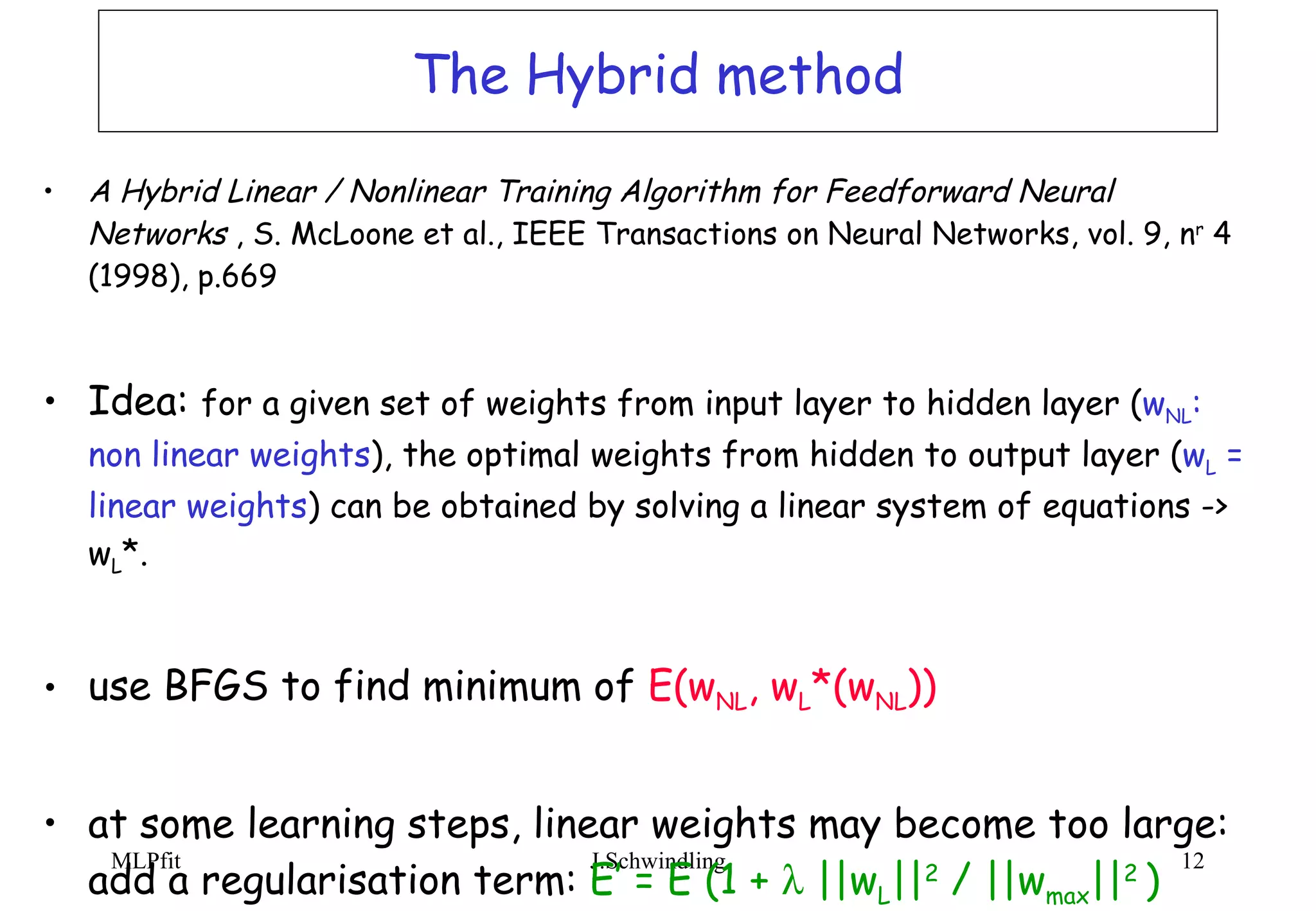
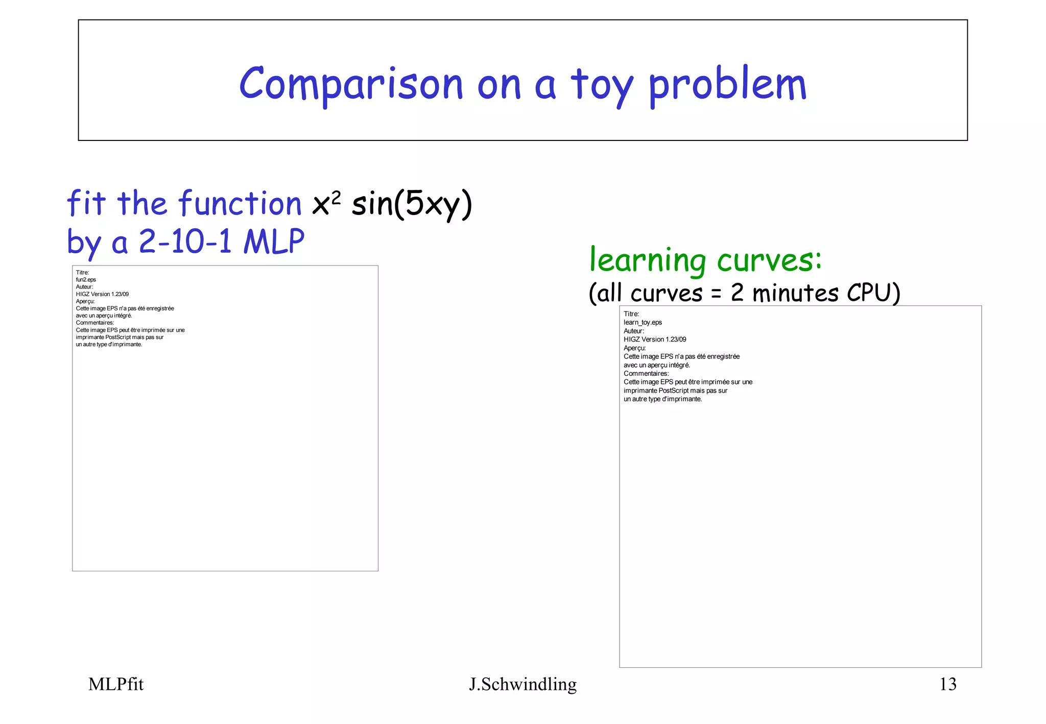
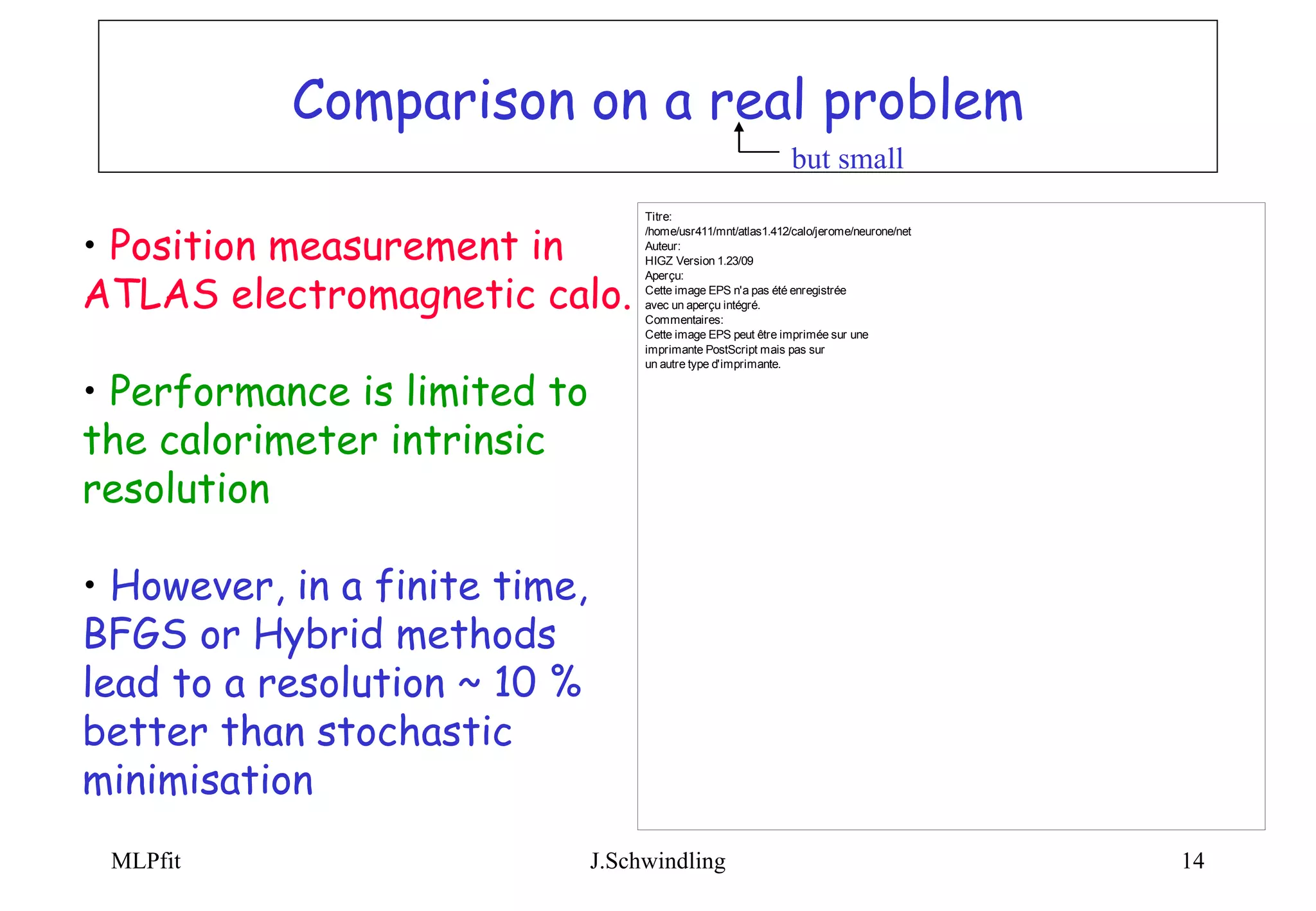
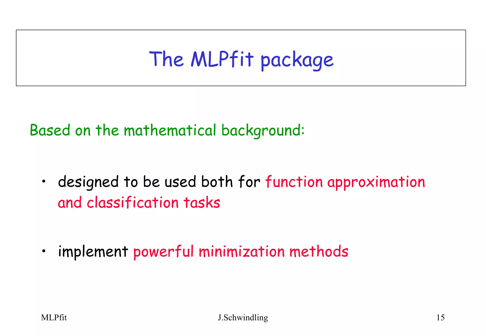
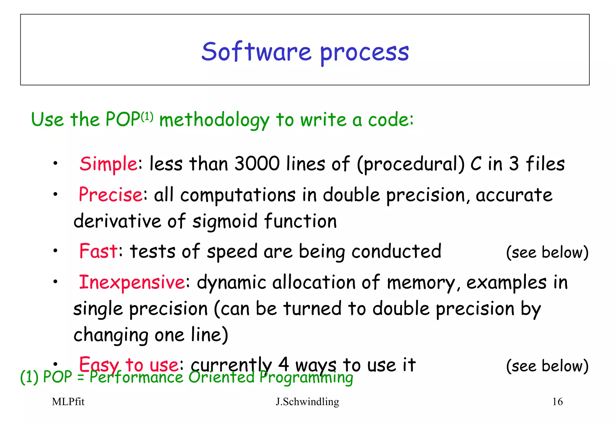
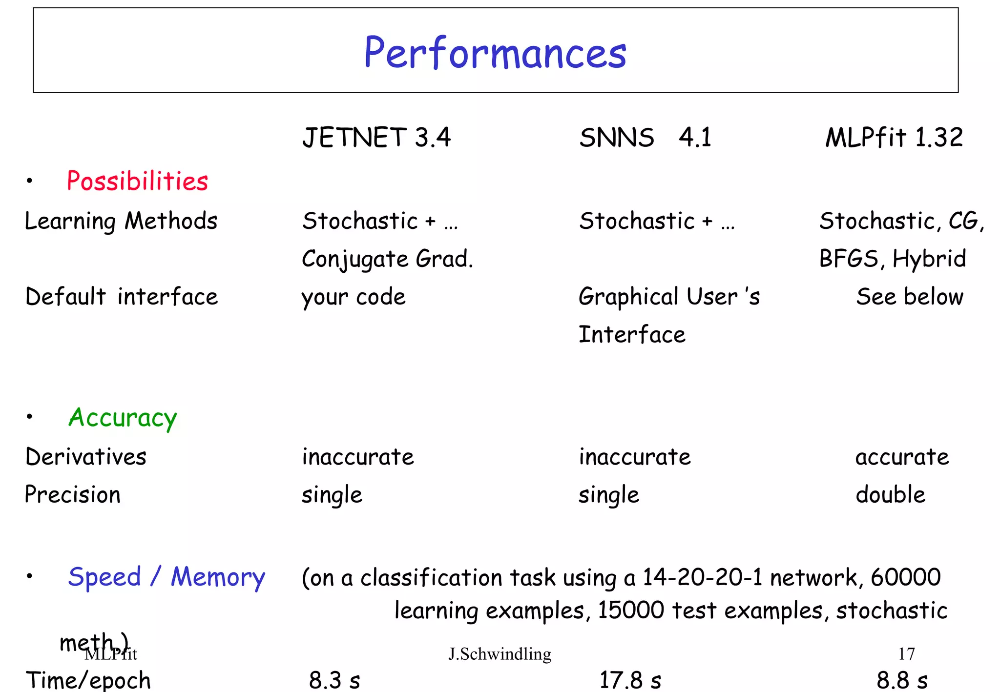
MLPfit is a tool for designing and training multi-layer perceptrons (MLPs) for tasks like function approximation and classification. It implements stochastic minimization as well as more powerful methods like conjugate gradients and BFGS. MLPfit is designed to be simple, precise, fast and easy to use for both standalone and integrated applications. Documentation and source code are available online.


![[update] Introductory Parts of the Book "Dive into Deep Learning"](https://cdn.slidesharecdn.com/ss_thumbnails/d2lq1introbasicssimplemodels-190415080926-thumbnail.jpg?width=640&height=640&fit=bounds)


