Downloaded 94 times


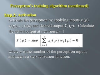
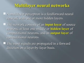
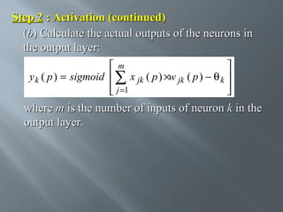
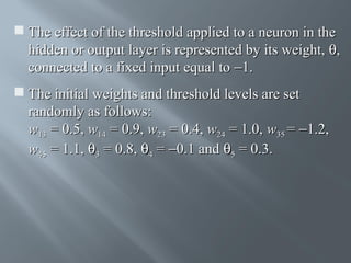
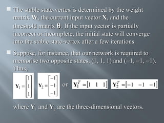
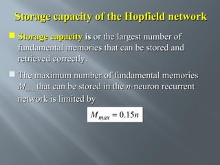
![How does the perceptron learn its classification
tasks?
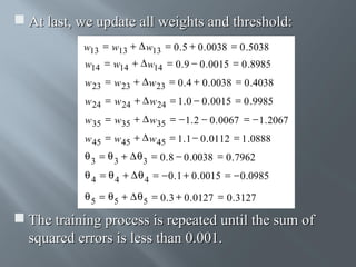
This is done by making small adjustments in the
weights to reduce the difference between the actual
and desired outputs of the perceptron. The initial
weights are randomly assigned, usually in the range
[−0.5, 0.5], and then updated to obtain the output
consistent with the training examples.](https://image.slidesharecdn.com/sctnnw-131126110438-phpapp01/85/SOFT-COMPUTERING-TECHNICS-Unit-1-20-320.jpg)
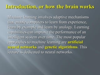
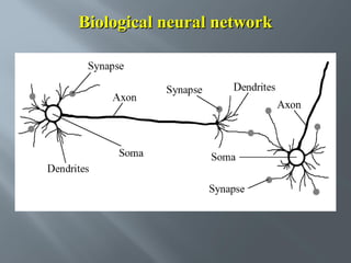
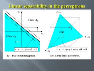
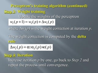
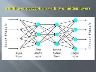
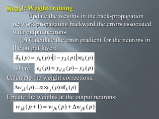
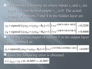
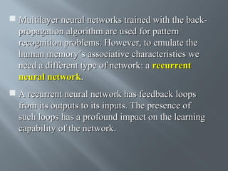
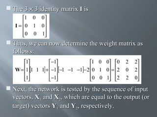
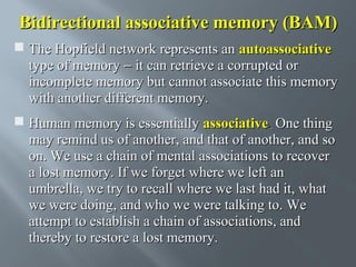
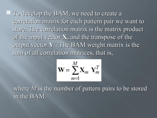
![Perceptron’s training algorithm
Step 1: Initialisation
Set initial weights w1, w2,…, wn and threshold
θ
to random numbers in the range [−0.5, 0.5].
If the error, e(p), is positive, we need to increase
perceptron output Y(p), but if it is negative, we
need to decrease Y(p).](https://image.slidesharecdn.com/sctnnw-131126110438-phpapp01/85/SOFT-COMPUTERING-TECHNICS-Unit-1-23-320.jpg)
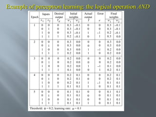
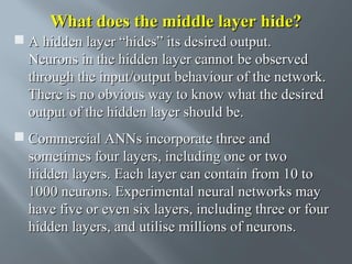
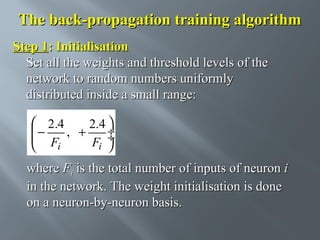
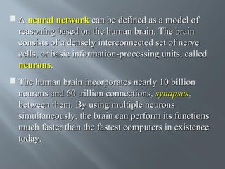
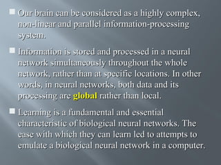
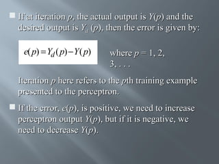
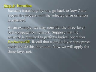
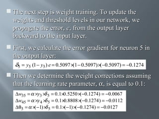
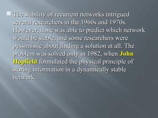
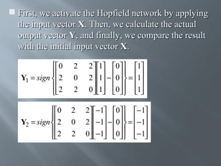
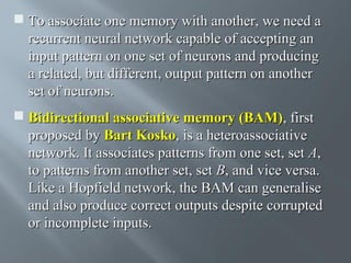
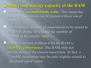
![Step 3: Weight training (continued)
(b) Calculate the error gradient for the neurons in
the hidden layer:
l
j ( p)
= y j ( p ) × 1 − y j ( p )] ×∑ k ( p ) w jk ( p )
[
k =1
Calculate the weight corrections:
∆wij ( p ) =
×xi ( p ) × j ( p )
Update the weights at the hidden neurons:
wij ( p + 1) = wij ( p ) + ∆wij ( p )](https://image.slidesharecdn.com/sctnnw-131126110438-phpapp01/85/SOFT-COMPUTERING-TECHNICS-Unit-1-38-320.jpg)
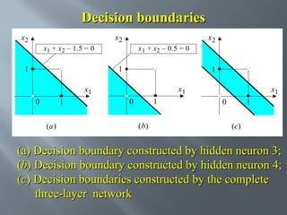


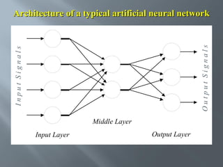
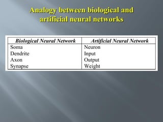
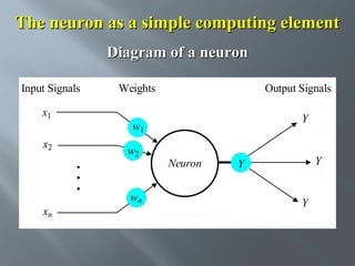
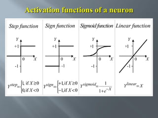
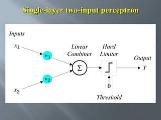
This document describes an artificial neural network project presented by Rm.Sumanth, P.Ganga Bashkar, and Habeeb Khan to Madina Engineering College. It provides an overview of artificial neural networks and supervised learning techniques. Specifically, it discusses the biological structure of neurons and how artificial neural networks emulate this structure. It then describes the perceptron model and learning rule, and how multilayer feedforward networks using backpropagation can learn more complex patterns through multiple layers of neurons.