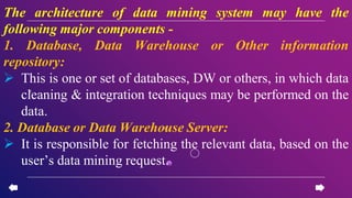
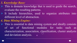
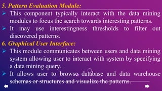
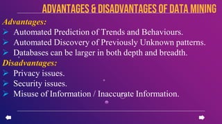
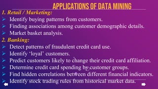
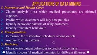
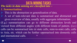
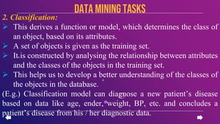
Download to read offline

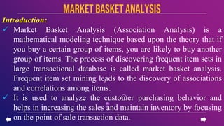


This document provides an introduction to data mining concepts including definitions, tasks, challenges, and techniques. It discusses data mining definitions, the data mining process including data preprocessing steps like cleaning, integration, transformation and reduction. It also covers common data mining tasks like classification, clustering, association rule mining and the Apriori algorithm. Overall, the document serves as a high-level overview of key data mining concepts and methods.