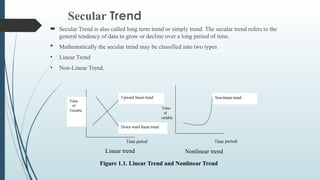
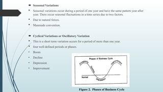
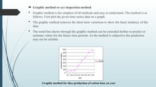
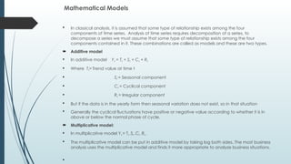
Time Series Analysis
Represented by :
1. Patil Ashwinee Prakash (CS041)
Introduction
 Definition :The numerical data which we get at different points of time-the set of observations-is
known as time series.
 A time series is a set of observations made at specified times and arranged in a chronological order.
 In time series analysis, current data in a series may be compared with past data in the same series.
 Uses of Time Series
 The analysis of time series is of great significance not only to the economists and business man but also
to the scientists, astronomists, geologists, sociologists, biologists, research worker etc. In the view of
following reasons
 It helps in understanding past behavior.
 It helps in planning future operations.
 It helps in evaluating current accomplishments.
 It facilitates comparison.
Secular Trend
 Secular Trend is also called long term trend or simply trend. The secular trend refers to the
general tendency of data to grow or decline over a long period of time.
 Mathematically the secular trend may be classified into two types
• Linear Trend
• Non-Linear Trend.
Linear trend
period
Nonlinear trend
Figure 1.1. Linear Trend and Nonlinear Trend
 Seasonal Variations
 Seasonal variations occur during a period of one year and have the same pattern year after
year. There occur seasonal fluctuations in a time series due to two factors.
 Due to natural forces.
 Manmade convention.
 Cyclical Variations or Oscillatory Variation
 This is a short term variation occurs for a period of more than one year.
 four well defined periods or phases.
• Boom
• Decline
• Depression
• Improvement
Figure 2. Phases of Business Cycle
 Graphic method or eye inspection method
 Graphic method is the simplest of all methods and easy to understand. The method is as
follows. First plot the given time series data on a graph.
 The graphic method removes the short term variations to show the basic tendency of the
data.
 The trend line drawn through the graphic method can be extended further to predict or
estimate values for the future time periods. As the method is subjective the prediction
may not be reliable.
Graphic method for thee production of cotton base on year
 Advantages
 It is very simplest method for study trend values and easy to draw trend.
 Sometimes the trend line drawn by the statistician experienced in computing trend
may be considered better than a trend line fitted by the use of a mathematical formula.
 Disadvantages:
 This method is highly subjective and curve varies from person to person who draws it.
 While drawing a trend line through this method a careful job has to be done.
 Method of Semi Averages
 This method is very simple and relatively objective as a freehand method. In this method, we
classify the time series data into two equal parts and then calculate Averages for each half. If the
data is for even number of years, it is easily divided into two.
 In this method, we can find the solution of a secular trend. For this, we have to show our time
series on graph paper. For example, we can take sales on X-axis and data of production on Y-axis.
 Advantages
 This method is simple to understand as compare to other methods for measuring the secular
trends.
 Everyone who applies this method will get the same result.
 Disadvantages
 The method assumes a straight line relationship between the plotted points without considering
the fact whether that relationship exists or not.
 Method of Moving Average:
 It is a method for computing trend values in a time series which eliminates the short term and
random fluctuations from the time series by means of moving average. Moving average of a period
m is a series of successive arithmetic means of m terms at a time starting with 1st
, 2nd
, 3rd
and so
on. The first average is the mean of first m terms.
 Advantages:
 This method is simple to under stand and easy to execute.
 It gives a correct picture of the long term trend if the trend is linear.
 Disadvantages:
 For a moving average of 2m+1, one does not get trend values for first m and last m periods.
 As the trend path does not correspond to any mathematical; function, it cannot be used for
forecasting or predicting values for future periods.
Mathematical Models
 In classical analysis, it is assumed that some type of relationship exists among the four
components of time series. Analysis of time series requires decomposition of a series, to
decompose a series we must assume that some type of relationship exists among the four
components contained in it. These combinations are called as models and these are two types.
 Additive model
 In additive model Yt = Tt + St + Ct + Rt
 Where Tt= Trend value at time t
 St = Seasonal component
 Ct = Cyclical component
 Rt = Irregular component
 But if the data is in the yearly form then seasonal variation does not exist, so in that situation
 Generally the cyclical fluctuations have positive or negative value according to whether it is in
above or below the normal phase of cycle.
 Multiplicative model:
 In multiplicative model Yt = Tt .St .Ct .Rt .
 The multiplicative model can be put in additive model by taking log both sides. The most business
analysis uses the multiplicative model and finds it more appropriate to analyze business situations.

SEASONAL VARIATIONS
Introduction
 Seasonal variations are regular and periodic variations having a period of
one year duration.
 The reason for determining seasonal variations in a time series is to isolate it
and to study its effect on the size of the variable in the index form which is
usually referred as seasonal index.
 Measurement of seasonal variations:
 There are different devices to measure the seasonal variations.
 Method of simple averages.
 Ratio to trend method .
 Ratio to moving average method.
Ratio to trend method:
 This method is an improvement over the simple averages method and this method
assumes a multiplicative model.
 The measurement of seasonal indices by this method consists of the following steps.
 Obtain the trend values by the least square method by fitting a mathematical curve,
either a straight line or second degree polynomial.
 Express the original data as the percentage of the trend values.
 The cyclical and irregular components are eliminated by averaging the percentages for
different months (quarters) if the data are In monthly (quarterly), thus leaving us with
indices of seasonal variations.
 Advantages:
 It is easy to compute and easy to understand.
 Compared with the method of monthly averages this method is certainly a more logical
procedure for measuring seasonal variations.
 Disadvantages:
 The main defect of the ratio to trend method is that if there are cyclical swings in the
series, the trend whether a straight line or a curve can never follow the actual data as
closely as a 12- monthly moving average does. So a seasonal index computed by the
ratio to moving average method may be less biased than the one calculated by the
ratio to trend method.
THANK YOU…..!

Business Statistics_Time Series1232.pptx

  • 1.
    Time Series Analysis Representedby : 1. Patil Ashwinee Prakash (CS041)
  • 2.
    Introduction  Definition :Thenumerical data which we get at different points of time-the set of observations-is known as time series.  A time series is a set of observations made at specified times and arranged in a chronological order.  In time series analysis, current data in a series may be compared with past data in the same series.  Uses of Time Series  The analysis of time series is of great significance not only to the economists and business man but also to the scientists, astronomists, geologists, sociologists, biologists, research worker etc. In the view of following reasons  It helps in understanding past behavior.  It helps in planning future operations.  It helps in evaluating current accomplishments.  It facilitates comparison.
  • 3.
    Secular Trend  SecularTrend is also called long term trend or simply trend. The secular trend refers to the general tendency of data to grow or decline over a long period of time.  Mathematically the secular trend may be classified into two types • Linear Trend • Non-Linear Trend. Linear trend period Nonlinear trend Figure 1.1. Linear Trend and Nonlinear Trend
  • 4.
     Seasonal Variations Seasonal variations occur during a period of one year and have the same pattern year after year. There occur seasonal fluctuations in a time series due to two factors.  Due to natural forces.  Manmade convention.  Cyclical Variations or Oscillatory Variation  This is a short term variation occurs for a period of more than one year.  four well defined periods or phases. • Boom • Decline • Depression • Improvement Figure 2. Phases of Business Cycle
  • 5.
     Graphic methodor eye inspection method  Graphic method is the simplest of all methods and easy to understand. The method is as follows. First plot the given time series data on a graph.  The graphic method removes the short term variations to show the basic tendency of the data.  The trend line drawn through the graphic method can be extended further to predict or estimate values for the future time periods. As the method is subjective the prediction may not be reliable. Graphic method for thee production of cotton base on year
  • 6.
     Advantages  Itis very simplest method for study trend values and easy to draw trend.  Sometimes the trend line drawn by the statistician experienced in computing trend may be considered better than a trend line fitted by the use of a mathematical formula.  Disadvantages:  This method is highly subjective and curve varies from person to person who draws it.  While drawing a trend line through this method a careful job has to be done.
  • 7.
     Method ofSemi Averages  This method is very simple and relatively objective as a freehand method. In this method, we classify the time series data into two equal parts and then calculate Averages for each half. If the data is for even number of years, it is easily divided into two.  In this method, we can find the solution of a secular trend. For this, we have to show our time series on graph paper. For example, we can take sales on X-axis and data of production on Y-axis.  Advantages  This method is simple to understand as compare to other methods for measuring the secular trends.  Everyone who applies this method will get the same result.  Disadvantages  The method assumes a straight line relationship between the plotted points without considering the fact whether that relationship exists or not.
  • 8.
     Method ofMoving Average:  It is a method for computing trend values in a time series which eliminates the short term and random fluctuations from the time series by means of moving average. Moving average of a period m is a series of successive arithmetic means of m terms at a time starting with 1st , 2nd , 3rd and so on. The first average is the mean of first m terms.  Advantages:  This method is simple to under stand and easy to execute.  It gives a correct picture of the long term trend if the trend is linear.  Disadvantages:  For a moving average of 2m+1, one does not get trend values for first m and last m periods.  As the trend path does not correspond to any mathematical; function, it cannot be used for forecasting or predicting values for future periods.
  • 9.
    Mathematical Models  Inclassical analysis, it is assumed that some type of relationship exists among the four components of time series. Analysis of time series requires decomposition of a series, to decompose a series we must assume that some type of relationship exists among the four components contained in it. These combinations are called as models and these are two types.  Additive model  In additive model Yt = Tt + St + Ct + Rt  Where Tt= Trend value at time t  St = Seasonal component  Ct = Cyclical component  Rt = Irregular component  But if the data is in the yearly form then seasonal variation does not exist, so in that situation  Generally the cyclical fluctuations have positive or negative value according to whether it is in above or below the normal phase of cycle.  Multiplicative model:  In multiplicative model Yt = Tt .St .Ct .Rt .  The multiplicative model can be put in additive model by taking log both sides. The most business analysis uses the multiplicative model and finds it more appropriate to analyze business situations. 
  • 10.
    SEASONAL VARIATIONS Introduction  Seasonalvariations are regular and periodic variations having a period of one year duration.  The reason for determining seasonal variations in a time series is to isolate it and to study its effect on the size of the variable in the index form which is usually referred as seasonal index.  Measurement of seasonal variations:  There are different devices to measure the seasonal variations.  Method of simple averages.  Ratio to trend method .  Ratio to moving average method.
  • 11.
    Ratio to trendmethod:  This method is an improvement over the simple averages method and this method assumes a multiplicative model.  The measurement of seasonal indices by this method consists of the following steps.  Obtain the trend values by the least square method by fitting a mathematical curve, either a straight line or second degree polynomial.  Express the original data as the percentage of the trend values.  The cyclical and irregular components are eliminated by averaging the percentages for different months (quarters) if the data are In monthly (quarterly), thus leaving us with indices of seasonal variations.  Advantages:  It is easy to compute and easy to understand.  Compared with the method of monthly averages this method is certainly a more logical procedure for measuring seasonal variations.  Disadvantages:  The main defect of the ratio to trend method is that if there are cyclical swings in the series, the trend whether a straight line or a curve can never follow the actual data as closely as a 12- monthly moving average does. So a seasonal index computed by the ratio to moving average method may be less biased than the one calculated by the ratio to trend method.
  • 12.