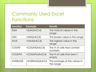
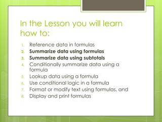
This document provides instructions for creating and modifying formulas in Microsoft Excel 2007. It covers referencing data, summarizing data using formulas, conditionally summarizing data, looking up data, using conditional logic, formatting text with formulas, and displaying and printing formulas. Specific topics covered include creating basic formulas, creating function formulas, commonly used functions like SUM, MIN, MAX, COUNT, AVERAGE, filtering and sorting lists, adding subtotals to lists, and removing filters and subtotals.

1. Microsoft
Excel 2007
Objective 3: Creating and
Modifying Formulas

2. In the Lesson you will learn
how to:
1. Reference data in formulas
2. Summarize data using formulas
3. Summarize data using subtotals
4. Conditionally summarize data using a
formula
5. Lookup data using a formula
6. Use conditional logic in a formula
7. Format or modify text using formulas, and
8. Display and print formulas

3. Summarize Data Using a
Formula
• Create a Basic Formula
• Create a Function Formula
• Commonly Used Excel Functions

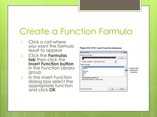
4. Create a Formula
1. Click the cell where you want to formula to
appear
2. Type =
3. Click a cell containing the first value you
want to include
 You may also enter a value manually
4. Type an operand such as +, -, /, or *
5. Click a cell containing the next value you
want to include
6. Enter operands and other cells or values as
necessary and press [Enter]

5. Create a Function Formula
1. Click a cell where
you want the formula
result to appear
2. Click the Formulas
tab then click the
Insert Function button
in the Function Library
group
3. In the Insert Function
dialog box select the
appropriate function
and click OK

6. Create a Function Formula
4. In the Function
Arguments dialog
box specify the
appropriate
settings or
cells, then click
OK

7. Commonly Used Excel
Functions
Function Example Results
SUM =SUM(A4:C4) The total of values in the
range
MIN =MIN(A4:C4) The lowest value in the range
MAX =MAX(A4:C4) The highest value in the
range
COUNT =COUNT(A4:C4) The # of cells that contain
numbers
COUNTA =COUNTA(A4:C4) The # of cells that aren’t
empty
AVERAGE =AVERAGE(A4:C4 The average of the values in
) the range

8. Summarize Data Using
Subtotals
Create, Filter, Sort, and Subtotal a list
Remove a Filter and Subtotals

9. Create a List
 Type related data in rows and
columns, with column headers describing
each columns data
 Type additional rows and columns as
needed making sure there are no empty
rows or columns between data

10. Filter a List
1. Click inside the list range
2. Click the Data tab then the Filter button
3. Click the list arrow at the top of the
column you want to filter
4. Click Select All to remove all check
marks
5. Click the check boxes for the items you
wish to display and click OK

11. Remove a Filter
1. Click inside the list
range
2. Click the Data tab
then the Filter
button to deselect
the button and
remove the Filter
arrows

12. Sort a List
1. Click inside the list
range
2. Click the Data tab
then the Sort button
3. In the Sort dialog
box choose what to
sort by and the
order
4. Add additional
levels if necessary
5. Click OK

13. Subtotal a List
1. Click the inside
the list range and
filter the list
2. Click the Subtotal
button on the
Data tab

14. Subtotal a List
3. In the Subtotal dialog
box click the At each
change in list arrow
then select the field
by which you sorted
4. Click the Use function
list arrow then click a
function to summarize
the data
 The functions that are
available are: SUM,
COUNT, AVERAGE,
MAX, and MIN

15. Remove Subtotals
 Click in the list range containing subtotals
 Click the Data tab then the Subtotal
button
 In the Subtotal dialog box click Remove
All

16. Lesson Review
 Open the Excel worksheet above named
Basic Formulas and complete to the best
of your ability