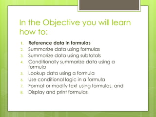
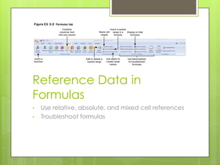
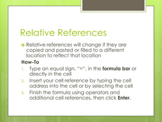
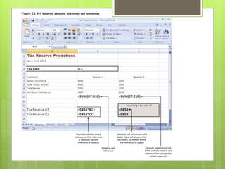
This document provides an overview of objectives and instructions for creating and modifying formulas in Microsoft Excel 2007. It covers topics such as: - Referencing data in formulas using relative, absolute, and mixed cell references, and troubleshooting formulas. - Summarizing data using formulas, subtotals, and conditional formulas. - Looking up data and using conditional logic in formulas. - Formatting or modifying text in formulas. - Displaying and printing formulas. 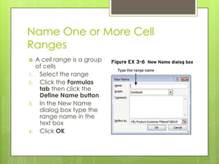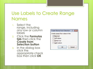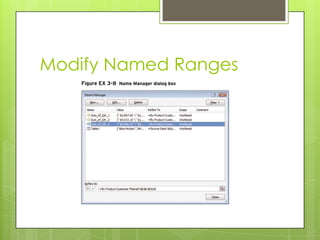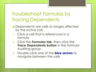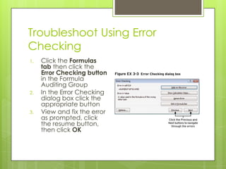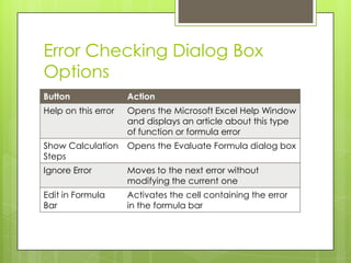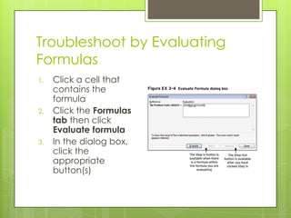The document provides step-by-step instructions for tasks like naming cell ranges, inserting named ranges in formulas, and troubleshooting formulas using the trace precedents and dependents buttons, error checking, and evaluating formulas.

1. Microsoft
Excel 2007
Objective 3: Creating and
Modifying Formulas

2. In the Objective you will learn
how to:
1. Reference data in formulas
2. Summarize data using formulas
3. Summarize data using subtotals
4. Conditionally summarize data using a
formula
5. Lookup data using a formula
6. Use conditional logic in a formula
7. Format or modify text using formulas, and
8. Display and print formulas

3. Reference Data in
Formulas
• Use relative, absolute, and mixed cell references
• Troubleshoot formulas

4. Relative References
 Relative references will change if they are
copied and pasted or filled to a different
location to reflect that location
How-To
1. Type an equal sign, “=“, in the formula bar or
directly in the cell
2. Insert your cell reference by typing the cell
address into the cell or by selecting the cell
3. Finish the formula using operators and
additional cell references, then click Enter.

5. Absolute References
 Absolute references will not change based on
where the “$” is located in the reference.
How-To
1. After entering the cell references, select the
cell reference, one at a time, that you want
to make an absolute reference and press F4
 The reference should now read $A$1
2. Press Enter or Tab

7. Troubleshoot Formulas by
Tracing Precedents
 Precedents are cells or ranges that affect
the active cell’s value.
1. Click a cell that contains a formula
2. Click the Formulas tab, then click the
Trace Precedents button in the Formula
Auditing group
3. Double-click one of the blue arrows to
navigate between the cell containing
the formula and the precedent cell(s)

8. Troubleshoot Formulas by
Tracing Dependents
 Dependents are cells or ranges affected
by the active cell.
1. Click a cell that is referenced in a
formula
2. Click the Formulas tab, then click the
Trace Dependents button in the Formula
Auditing group
3. Double-click one of the blue arrows to
navigate between the cells

9. Troubleshoot by
Tracing, Locating and
Resolving Errors
1. Click the cell that shows the error
 Common errors are shown on the next slide
2. Click the Formulas tab, click the Error
Checking list arrow in the Formula
Auditing group, then click Trace Error
3. Make edits to the formula in the formula
bar

10. Common Errors
Error Means
#DIV/0! Value is divided by zero
#NAME? Excel does not recognize text
#N/A Value is not available for the formula
#NULL! Formula specifies an intersection of two areas
that do not intersect
#NUM! Invalid formula number(s)
#REF! Invalid cell reference
#VALUE! Operand or argument is incorrect

11. Troubleshoot Using Error
Checking
1. Click the Formulas
tab then click the
Error Checking button
in the Formula
Auditing Group
2. In the Error Checking
dialog box click the
appropriate button
3. View and fix the error
as prompted, click
the resume button,
then click OK

12. Error Checking Dialog Box
Options
Button Action
Help on this error Opens the Microsoft Excel Help Window
and displays an article about this type
of function or formula error
Show Calculation Opens the Evaluate Formula dialog box
Steps
Ignore Error Moves to the next error without
modifying the current one
Edit in Formula Activates the cell containing the error
Bar in the formula bar

13. Troubleshoot by Evaluating
Formulas
1. Click a cell that
contains the
formula
2. Click the Formulas
tab then click
Evaluate formula
3. In the dialog box,
click the
appropriate
button(s)

14. Using References to Data in
Other Worksheets
 If necessary, open the workbook containing
the data
 In the current workbook:
1. Click the cell that will contain the formula and
type =
2. Click the workbook, or worksheet, containing
the value you want to include and click the
cell
3. Type an operand (such as + or -) to continue
the formula and select other cells as necessary
4. Press [Enter]

15. Name One or More Cell
Ranges
 A cell range is a group
of cells
1. Select the range
2. Click the Formulas
tab then click the
Define Name button
3. In the New Name
dialog box type the
range name in the
text box
4. Click OK

16. Use Labels to Create Range
Names
1. Select the
range, including
any row or column
labels
2. Click the Formulas
tab then click the
Create from
Selection button
3. In the dialog box
click the
appropriate check
box then click OK

17. Modify Named Ranges

18. Insert a Named Range in a
Formula
1. Click in the cell where the formula will
appear and begin typing the formula
2. When you need to insert the named
range, click the Formulas tab, the Use in
Formula button, then the range name in
the drop-down menu
3. Complete the formula as appropriate

19. Lesson Review
 Complete the Get to know Excel 2007 –
Enter formulas activity above this
presentation.