DATA-ANALYSIS-AND-INTERPRETATION-pptx

1. Agenda
• Introduction to Excel Interface
• Basic Functions (SUM, COUNT, AVERAGE, etc.)
• Text Functions and Dates
• Lookup and Conditional Functions
• Data Cleaning Techniques
• Data Visualization with Conditional Formatting
• Sorting, Filtering, and Subtotals
• Working with Ranges and Tables
• Q&A and Practical Exercises

2. Microsoft Excel Overview
• Spreadsheet software for data organization and analysis.
• Offers data analysis, visualization, storage, and management.
Importance in Data Analysis:
• Data preparation and cleaning.
• Basic and advanced data analysis.
• Data visualization for trends and patterns.
• Data sharing in a commonly accepted format.
Importance of Understanding Excel Interface:
• Efficiency in navigation and task execution.
• Improved data access and utilization.
• Reduced risk of errors.
• Customization for specific needs.

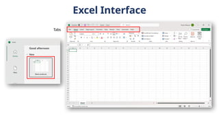
3. Excel Interface
• Excel's user environment for data work.
• Key elements include the Ribbon, Tabs, and Quick Access Toolbar.
The Ribbon:
• Horizontal strip with tabs and groups of commands.
• Tabs like Home, Insert, Page Layout, etc.
Quick Access Toolbar:
• Customizable toolbar for quick access to common commands.
Various Views:
• Normal View: Default for data entry.
• Page Layout View: Shows print layout.
• Page Break Preview: Reveals print page breaks.

4. Excel Interface
Tabs

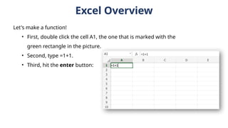
5. Excel Overview
Let's make a function!
• First, double click the cell A1, the one that is marked with the
green rectangle in the picture.
• Second, type =1+1.
• Third, hit the enter button:

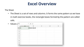
6. The Sheet
• The Sheet is a set of rows and columns. It forms the same pattern as we have
in math exercise books, the rectangle boxes formed by the pattern are called
cells.
• Values can be typed to cells.
Excel Overview

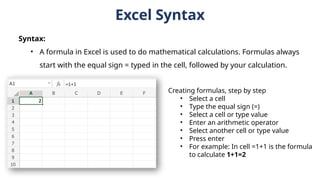
7. Syntax:
• A formula in Excel is used to do mathematical calculations. Formulas always
start with the equal sign = typed in the cell, followed by your calculation.
Excel Syntax
Creating formulas, step by step
• Select a cell
• Type the equal sign (=)
• Select a cell or type value
• Enter an arithmetic operator
• Select another cell or type value
• Press enter
• For example: In cell =1+1 is the formula
to calculate 1+1=2

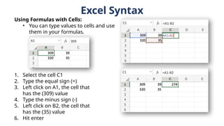
8. Using Formulas with Cells:
• You can type values to cells and use
them in your formulas.
1. Select the cell C1
2. Type the equal sign (=)
3. Left click on A1, the cell that
has the (309) value
4. Type the minus sign (-)
5. Left click on B2, the cell that
has the (35) value
6. Hit enter
Excel Syntax

9. Excel Fill
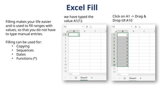
Filling makes your life easier
and is used to fill ranges with
values, so that you do not have
to type manual entries.
Filling can be used for:
• Copying
• Sequences
• Dates
• Functions (*)
we have typed the
value A1(1):
Click on A1 -> Drag &
Drop till A10

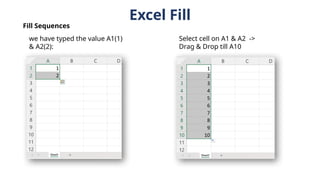
10. Excel Fill
we have typed the value A1(1)
& A2(2):
Select cell on A1 & A2 ->
Drag & Drop till A10
Fill Sequences

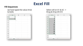
11. Excel Fill
we have typed the value A1(2)
& A2(4):
Select cell on A1 & A2 ->
Drag & Drop till A10
Fill Sequences

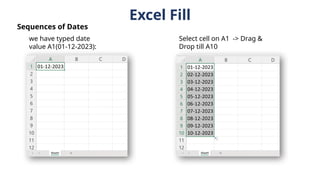
12. Excel Fill
we have typed date
value A1(01-12-2023):
Select cell on A1 -> Drag &
Drop till A10
Sequences of Dates

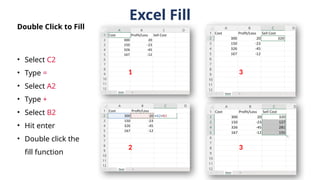
13. Excel Fill
• Select C2
• Type =
• Select A2
• Type +
• Select B2
• Hit enter
• Double click the
fill function
Double Click to Fill
1
2
3
3

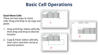
14. Basic Cell Operations
Excel Move Cells
There are two ways to move
cells: Drag and drop or by copy and
paste.
1. Drag and Drop: Select cell/cells,
then drop and drop to desired
location
2. Copy & Paste: Select cell/cells,
then ctrl+x and then ctrl+p at
desired location
1
2
3

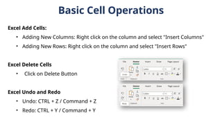
15. Basic Cell Operations
Excel Add Cells:
• Adding New Columns: Right click on the column and select "Insert Columns"
• Adding New Rows: Right click on the column and select "Insert Rows"
Excel Delete Cells
• Click on Delete Button
Excel Undo and Redo
• Undo: CTRL + Z / Command + Z
• Redo: CTRL + Y / Command + Y

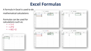
16. Excel Formulas
A formula in Excel is used to do
mathematical calculations
Formulas can be used for
calculations such as:
• = 1+1
• = 2*2
• = 4/2 =2

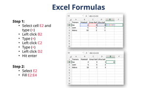
17. Excel Formulas
Step 1:
• Select cell E2 and
type (=)
• Left click B2
• Type (+)
• Left click C2
• Type (+)
• Left click D2
• Hit enter
Step 2:
• Select E2
• Fill E2:E4

18. Excel Formulas
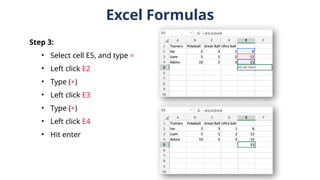
Step 3:
• Select cell E5, and type =
• Left click E2
• Type (+)
• Left click E3
• Type (+)
• Left click E4
• Hit enter

19. Basic Excel Functions
Dataset: customer_shopping_data

20. Basic Excel Functions
SUM Function:
• Purpose: Adds up a range of numbers.
• Usage: = SUM(range)
• Example: =SUM(A1:A5) adds the values in cells A1 through A5.

21. Basic Excel Functions
SUMIF Function:
• Purpose: Adds numbers in a range based on a specific condition.
• Usage: = SUMIF(range, criteria, [sum_range])
• Example: = SUMIF(A1:A5, ">10") sums values in A1 to A5 that are greater
than 10.

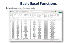
22. Basic Excel Functions
COUNT Function:
• Purpose: Counts the number of cells that contain numbers.
• Usage: =COUNT(range)
• Example: =COUNT(A1:A5) counts how many cells in A1 to A5 contain
numbers.

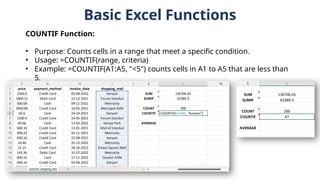
23. Basic Excel Functions
COUNTIF Function:
• Purpose: Counts cells in a range that meet a specific condition.
• Usage: =COUNTIF(range, criteria)
• Example: =COUNTIF(A1:A5, "<5") counts cells in A1 to A5 that are less than
5.

24. Basic Excel Functions
AVERAGE Function:
• Purpose: Calculates the average of a range of numbers.
• Usage: =AVERAGE(range)
• Example: =AVERAGE(A1:A5) calculates the average of values in A1 to A5.

25. Text Functions
FIND Function:
• Purpose: Finds the position of a substring within a text string.
• Usage: = FIND(find_text, within_text, [start_num])
• Example: = FIND("apple", "I have an apple") returns 13 because it finds
"apple" starting at the 13th character in the text.

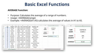
26. Text Functions
CONCATENATE Function (or & Operator):
• Purpose: Combines multiple text strings into one.
• Usage: =CONCATENATE(text1, text2, ...), or you can simply use the &
operator to combine text.

27. Text Functions
LEN Function:
• Purpose: Counts the number of characters in a text string.
• Usage: =LEN(text)
• Example: =LEN("Hello, world!") returns 13 because the text contains 13
characters.

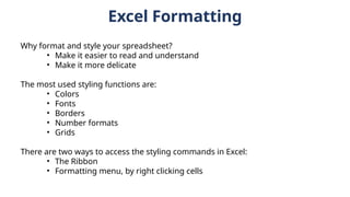
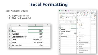
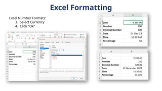
28. Excel Formatting
Why format and style your spreadsheet?
• Make it easier to read and understand
• Make it more delicate
The most used styling functions are:
• Colors
• Fonts
• Borders
• Number formats
• Grids
There are two ways to access the styling commands in Excel:
• The Ribbon
• Formatting menu, by right clicking cells

29. Excel Formatting
Styling Commands in Ribbon

30. Excel Formatting
Styling Commands, Right
Clicking Cells
Format Painter

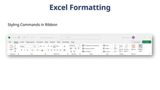
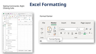
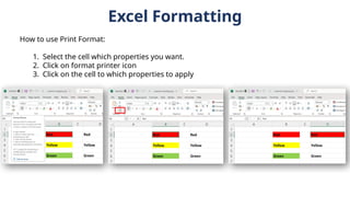
31. Excel Formatting
How to use Print Format:
1. Select the cell which properties you want.
2. Click on format printer icon
3. Click on the cell to which properties to apply

32. Excel Formatting
Excel Number Formats:
1. Right Click on cell
2. Click on Format Cell

33. Excel Formatting
Excel Number Formats:
3. Select Currency
4. Click "Ok"

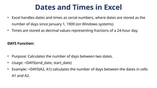
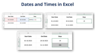
34. Dates and Times in Excel
• Excel handles dates and times as serial numbers, where dates are stored as the
number of days since January 1, 1900 (on Windows systems).
• Times are stored as decimal values representing fractions of a 24-hour day.
DAYS Function:
• Purpose: Calculates the number of days between two dates.
• Usage: =DAYS(end_date, start_date)
• Example: =DAYS(A2, A1) calculates the number of days between the dates in cells
A1 and A2.

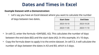
35. Dates and Times in Excel
Example Dataset with a Demonstration:
• Let's say you have an Excel dataset where you want to calculate the number
of days between two dates. Start Date End Date
2023-10-10 2023-10-20
2023-11-05 2023-11-10
• In cell C2, enter the formula =DAYS(B2, A2). This calculates the number of days
between the end date (B2) and the start date (A2). In this example, it's 10 days.
• Copy the formula down to apply it to the entire dataset. In cell C3, it will calculate the
number of days between the dates in A3 and B3, which is 5 days.

36. Dates and Times in Excel

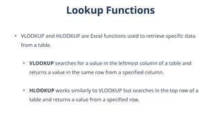
37. Lookup Functions
• VLOOKUP and HLOOKUP are Excel functions used to retrieve specific data
from a table.
• VLOOKUP searches for a value in the leftmost column of a table and
returns a value in the same row from a specified column.
• HLOOKUP works similarly to VLOOKUP but searches in the top row of a
table and returns a value from a specified row.

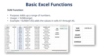
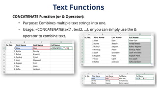
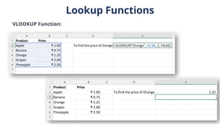
38. Lookup Functions
How to Use VLOOKUP and HLOOKUP:
VLOOKUP Function:
• Usage: =VLOOKUP(lookup_value, table_array, col_index_num,
[range_lookup])
• lookup_value is the value you want to find.
• table_array is the range containing the data you want to search.
• col_index_num is the column number from which to return data.
• [range_lookup] is optional and can be set to FALSE for an exact match or
TRUE for an approximate match (usually set to FALSE for most cases).

39. Lookup Functions
VLOOKUP Function:

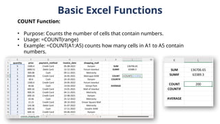
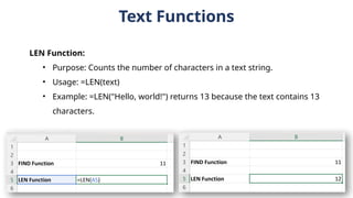
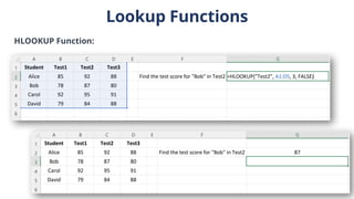
40. Lookup Functions
HLOOKUP Function:
• Usage: = HLOOKUP(lookup_value, table_array, row_index_num,
[range_lookup])
• lookup_value is the value you want to find.
• table_array is the range containing the data you want to search.
• row_index_num is the row number from which to return data.
• [range_lookup] works the same way as in VLOOKUP.

41. Lookup Functions
HLOOKUP Function:

42. Conditional Functions
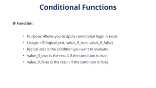
IF Function:
• Purpose: Allows you to apply conditional logic in Excel.
• Usage: =IF(logical_test, value_if_true, value_if_false)
• logical_test is the condition you want to evaluate.
• value_if_true is the result if the condition is true.
• value_if_false is the result if the condition is false.

43. Conditional Functions

44. Conditional Functions
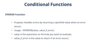
IFERROR Function:
• Purpose: Handles errors by returning a specified value when an error
occurs.
• Usage: =IFERROR(value, value_if_error)
• value is the expression or formula you want to evaluate.
• value_if_error is the value to return if an error occurs.

45. Conditional Functions

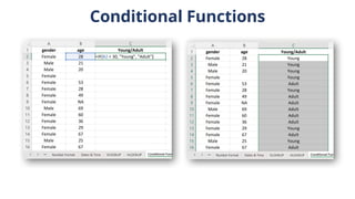
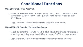
46. Conditional Functions
Using IF Function for Pass/Fail:
• In cell C2, enter the formula: =IF(B2 >= 50, "Pass", "Fail"). This checks if the
score in cell B2 is greater than or equal to 50 and returns "Pass" or "Fail"
accordingly.
• Copy this formula down the column to apply it to all students.
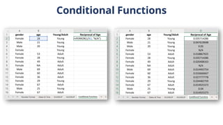
Using IFERROR Function for Handling Errors:
• In cell D2, enter the formula: =IFERROR(B2, "N/A"). This checks if there is an
error (e.g., a missing score in cell B2) and returns "N/A" if an error occurs.
• Copy this formula down the column to handle errors for all students.

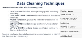
47. Data Cleaning Techniques
Text Functions and Their Role in Cleaning Data:
• TRIM Function: Removes leading/trailing spaces, improving
formatting.
• LOWER and UPPER Functions: Standardize text to lowercase or
uppercase.
• PROPER Function: Capitalize the first letter of each word for
consistency.
• CONCATENATE Function: Merge text from multiple cells for
uniformity.
• LEFT and RIGHT Functions: Extract specific text portions for
cleaning and analysis.
Suppose you have a dataset of product names, and you want to clean the
text data to ensure consistency:
Product Name
Apple iPhone 12
Samsung Galaxy S21
hp Laptop
Dell XPS 15 Laptop
Microsoft Surface Pro 7
ASUS ZenBook

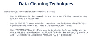
48. Data Cleaning Techniques
Here's how you can use text functions for data cleaning:
• Use the TRIM Function: In a new column, use the formula =TRIM(A2) to remove extra
spaces from the product names.
• Use the PROPER Function: In another new column, use the formula =PROPER(B2) to
capitalize the first letter of each word in the cleaned product names.
• Use CONCATENATE Function: If you want to standardize the format further, you can
concatenate the cleaned text with additional information. For example, if you want to
add " - Electronics" to each product name, use =B2 & " - Electronics".

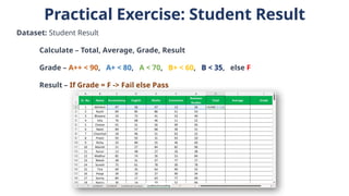
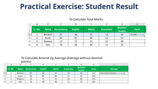
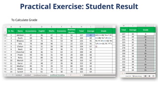
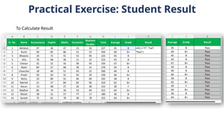
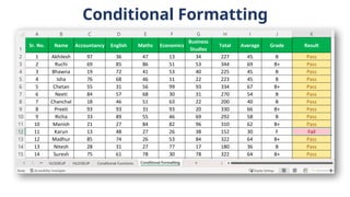
49. Practical Exercise: Student Result
Dataset: Student Result
Calculate – Total, Average, Grade, Result
Grade – A++ < 90, A+ < 80, A < 70, B+ < 60, B < 35, else F
Result – If Grade = F -> Fail else Pass

50. Practical Exercise: Student Result
To Calculate Total Marks
To Calculate Around Up Average (Average without decimal
points)

51. Practical Exercise: Student Result
To Calculate Grade

52. Practical Exercise: Student Result
To Calculate Result

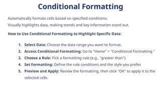
53. Conditional Formatting
Automatically formats cells based on specified conditions.
Visually highlights data, making trends and key information stand out.
How to Use Conditional Formatting to Highlight Specific Data:
1. Select Data: Choose the data range you want to format.
2. Access Conditional Formatting: Go to "Home" > "Conditional Formatting."
3. Choose a Rule: Pick a formatting rule (e.g., "greater than").
4. Set Formatting: Define the rule conditions and the style you prefer.
5. Preview and Apply: Review the formatting, then click "OK" to apply it to the
selected cells.

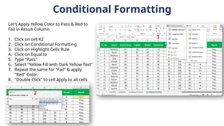
54. Conditional Formatting
Let's Apply Yellow Color to Pass & Red to
Fail in Result Column
1. Click on cell K2
2. Click on Conditional Formatting
3. Click on Highlight Cells Rule
4. Click on Equal to
5. Type "Pass"
6. Select "Yellow Fill with Dark Yellow Text"
7. Repeat the same for "Fail" & apply
"Red" Color.
8. "Double Click" to cell apply to all cells
1
2

55. Conditional Formatting

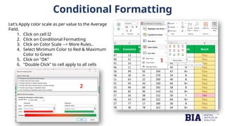
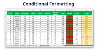
56. Conditional Formatting
Let's Apply color scale as per value to the Average
Field.
1. Click on cell I2
2. Click on Conditional Formatting
3. Click on Color Scale --> More Rules..
4. Select Minimum Color to Red & Maximum
Color to Green
5. Click on "OK"
6. "Double Click" to cell apply to all cells
1
2

57. Conditional Formatting

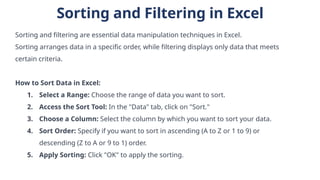
58. Sorting and Filtering in Excel
Sorting and filtering are essential data manipulation techniques in Excel.
Sorting arranges data in a specific order, while filtering displays only data that meets
certain criteria.
How to Sort Data in Excel:
1. Select a Range: Choose the range of data you want to sort.
2. Access the Sort Tool: In the "Data" tab, click on "Sort."
3. Choose a Column: Select the column by which you want to sort your data.
4. Sort Order: Specify if you want to sort in ascending (A to Z or 1 to 9) or
descending (Z to A or 9 to 1) order.
5. Apply Sorting: Click "OK" to apply the sorting.

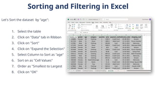
59. Sorting and Filtering in Excel
Let's Sort the dataset by "age":
1. Select the table
2. Click on "Data" tab in Ribbon
3. Click on "Sort"
4. Click on "Expand the Selection"
5. Select Column to Sort as "age"
6. Sort on as "Cell Values"
7. Order as "Smallest to Largest
8. Click on "OK"

60. Sorting and Filtering in Excel

61. Sorting and Filtering in Excel
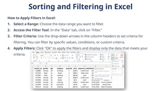
How to Apply Filters in Excel:
1. Select a Range: Choose the data range you want to filter.
2. Access the Filter Tool: In the "Data" tab, click on "Filter."
3. Filter Criteria: Use the drop-down arrows in the column headers to set criteria for
filtering. You can filter by specific values, conditions, or custom criteria.
4. Apply Filters: Click "OK" to apply the filters and display only the data that meets your
criteria.

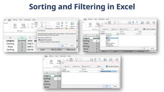
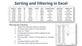
62. Sorting and Filtering in Excel
Filtering the Columns:
1. Select the Top row (column names)
2. In Home Tab, click on "Sort & Filter"
3. Click on "Filter"
4. A drop-down button will be added to the
column names.
5. For Example – Click on Drop-down at "Gender
Col"
6. Unselect Male & click "OK"
7. This will show only Female Customers

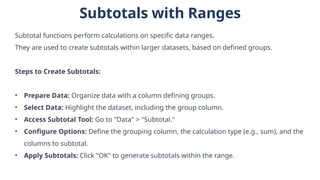
63. Subtotals with Ranges
Subtotal functions perform calculations on specific data ranges.
They are used to create subtotals within larger datasets, based on defined groups.
Steps to Create Subtotals:
• Prepare Data: Organize data with a column defining groups.
• Select Data: Highlight the dataset, including the group column.
• Access Subtotal Tool: Go to "Data" > "Subtotal."
• Configure Options: Define the grouping column, the calculation type (e.g., sum), and the
columns to subtotal.
• Apply Subtotals: Click "OK" to generate subtotals within the range.

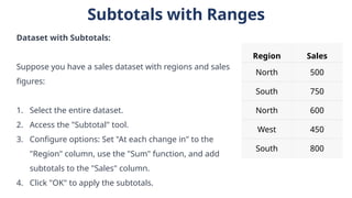
64. Subtotals with Ranges
Dataset with Subtotals:
Suppose you have a sales dataset with regions and sales
figures:
1. Select the entire dataset.
2. Access the "Subtotal" tool.
3. Configure options: Set "At each change in" to the
"Region" column, use the "Sum" function, and add
subtotals to the "Sales" column.
4. Click "OK" to apply the subtotals.
Region Sales
North 500
South 750
North 600
West 450
South 800

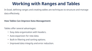
65. Working with Ranges and Tables
In Excel, defining ranges and creating tables are techniques to structure and manage
data effectively.
How Tables Can Improve Data Management:
Tables offer several advantages:
• Easy data organization with headers.
• Auto-expansion for new data.
• Built-in filtering and sorting options.
• Improved data integrity and error reduction.

66. Working with Ranges and Tables
Demonstration of Defining a Table:
1. Select Data: Highlight the data range you want to convert into a table.
2. Create a Table: In the "Insert" tab, click on "Table."
3. Define the Table: Ensure the "Create Table" dialog recognizes your data
range. Check the box if your table has headers.
4. Confirm: Click "OK" to create the table.

67. Thank You!!!