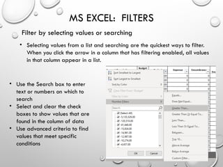
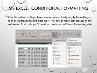
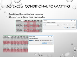
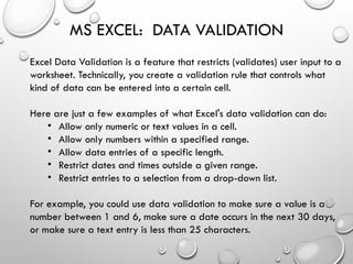
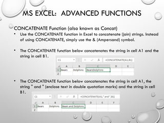
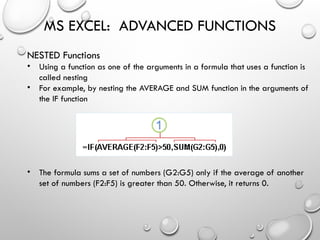
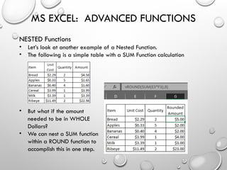
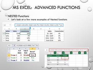
STEPPING IT UP
WITH
MICROSOFT
EXCEL
STEPPING
IT UP
TOPICS
• FILTERS
• CONDITIONAL FORMATTING
• DATA VALIDATION
• ADVANCED FUNCTIONS
• VLOOKUP
• LEFT, RIGHT
• SUBTOTAL
• CONCAT
• NESTED FUNCTIONS
• MATHEMATICAL
• CONDITIONAL
MS EXCEL: FILTERS
• Filters can be used to narrow down the “Clean” data in your
worksheet and hide parts of it from view. Filtering allows you
to qualify and display only the data that interests you.
• Use AutoFilter or built-in comparison operators like "greater
than" and “top 10” in Excel to show the data you want and
hide the rest. Once you filter data in a range of cells or
table, you can either reapply a filter to get up-to-date results
or clear a filter to redisplay all the data.
• By filtering information in a worksheet, you can find values
quickly. You can filter on one or more columns of data. With
filtering, you can control not only what you want to see, but
what you want to exclude.
MS EXCEL: FILTERS
• Select a cell within your data table, then under the Data
Ribbon, choose Filter. Once the Filter toggle is selected, small
arrows will appear on the column headers.
• Choose the column you want to filter and click the drop-down
arrow.
MS EXCEL: FILTERS
Filter by selecting values or searching
• Selecting values from a list and searching are the quickest ways to filter.
When you click the arrow in a column that has filtering enabled, all values
in that column appear in a list.
• Use the Search box to enter
text or numbers on which to
search
• Select and clear the check
boxes to show values that are
found in the column of data
• Use advanced criteria to find
values that meet specific
conditions
MS EXCEL: CONDITIONAL FORMATTING
Conditional formatting allows you to automatically apply formatting—
such as colors, icons, and data bars—to one or more cells based on the
cell value. To do this, you'll need to create a conditional formatting rule.
MS EXCEL: CONDITIONAL FORMATTING
• Conditional formatting box appears.
• Choose your criteria. See your results.
MS EXCEL: DATA VALIDATION
Excel Data Validation is a feature that restricts (validates) user input to a
worksheet. Technically, you create a validation rule that controls what
kind of data can be entered into a certain cell.
Here are just a few examples of what Excel's data validation can do:
• Allow only numeric or text values in a cell.
• Allow only numbers within a specified range.
• Allow data entries of a specific length.
• Restrict dates and times outside a given range.
• Restrict entries to a selection from a drop-down list.
For example, you could use data validation to make sure a value is a
number between 1 and 6, make sure a date occurs in the next 30 days,
or make sure a text entry is less than 25 characters.
MS EXCEL: DATA VALIDATION
One example is that data validation can be used to present the user
with a predefined choice in a dropdown menu:
Data validation is defined in a
window with 3 tabs: Settings, Input
Message, and Error Alert:
MS EXCEL: ADVANCED FUNCTIONS
VLOOKUP
• VLOOKUP is one of the most widely used functions in Excel. VLOOKUP lets
you look up a value in a column on the left, then returns information in
another column to the right if it finds a match. VLOOKUP supports
approximate and exact matching, and wildcards (* ?) for partial matches.
• VLOOKUP function says:
MS EXCEL: ADVANCED FUNCTIONS
VLOOKUP
• V is for vertical
• The purpose of VLOOKUP is to get information from a table organized like
this
• Using the Order number in column B as a lookup value, VLOOKUP can get
the Customer ID, Amount, Name, or State for any order.
• VLOOKUP can only look to the right in the data. The data you want to
retrieve (result values) can appear in any column to the right of the lookup
values
MS EXCEL: ADVANCED FUNCTIONS
LEFT, RIGHT Functions
• The Excel LEFT and RIGHT functions extracts a given number of characters
from the left or right side of a supplied text string.
• Use the LEFT function when you want to extract characters starting at the left
side of text.
• LEFT or RIGHT will extract digits from numbers as well.
MS EXCEL: ADVANCED FUNCTIONS
SUBTOTAL Function
• The Excel SUBTOTAL function provides a subtotal of values in a list of data.
The SUBTOTAL function can return a SUM, AVERAGE, COUNT, MAX, and
others and the function can either include or exclude values in hidden rows.
• SUBTOTAL behavior is controlled by the
function_num argument, which is
provided as a numeric value. There are
11 functions available, each with two
options.
1. function_num - A number that specifies which function to use in calculating subtotals within a list
2. ref1 - A named range or reference to subtotal
3. ref2 - [optional] A named range or reference to subtotal
MS EXCEL: ADVANCED FUNCTIONS
SUBTOTAL Function
• When function_num is between 1-11, SUBTOTAL includes values that are
hidden
• When function_num is between 101-111, SUBTOTAL excludes values that
are hidden
• SUBTOTAL is designed to work with vertical data values arranged vertically.
In horizontal ranges, values in hidden columns are always included.
• In filtered lists, SUBTOTAL always ignores values in hidden rows, regardless
of function_num.
Personal recommendation:
Use SUBTOTAL at the top
of your data, especially if
in conjunction with Filters.
MS EXCEL: ADVANCED FUNCTIONS
CONCATENATE Function (also known as Concat)
• Use the CONCATENATE function in Excel to concatenate (join) strings. Instead
of using CONCATENATE, simply use the & (Ampersand) symbol.
• The CONCATENATE function below concatenates the string in cell A1 and the
string in cell B1.
• The CONCATENATE function below concatenates the string in cell A1, the
string " and " (enclose text in double quotation marks) and the string in cell
B1.
MS EXCEL: ADVANCED FUNCTIONS
NESTED Functions
• Using a function as one of the arguments in a formula that uses a function is
called nesting
• For example, by nesting the AVERAGE and SUM function in the arguments of
the IF function
• The formula sums a set of numbers (G2:G5) only if the average of another
set of numbers (F2:F5) is greater than 50. Otherwise, it returns 0.
MS EXCEL: ADVANCED FUNCTIONS
NESTED Functions
• Let’s look at another example of a Nested Function.
• The following is a simple table with a SUM Function calculation
• But what if the amount
needed to be in WHOLE
Dollars?
• We can nest a SUM function
within a ROUND function to
accomplish this in one step.
MS EXCEL: ADVANCED FUNCTIONS
NESTED Functions
• Let’s look at a few more examples of Nested functions

This is a presentation on Microsoft Excel

  • 1.
  • 2.
    STEPPING IT UP TOPICS • FILTERS •CONDITIONAL FORMATTING • DATA VALIDATION • ADVANCED FUNCTIONS • VLOOKUP • LEFT, RIGHT • SUBTOTAL • CONCAT • NESTED FUNCTIONS • MATHEMATICAL • CONDITIONAL
  • 3.
    MS EXCEL: FILTERS •Filters can be used to narrow down the “Clean” data in your worksheet and hide parts of it from view. Filtering allows you to qualify and display only the data that interests you. • Use AutoFilter or built-in comparison operators like "greater than" and “top 10” in Excel to show the data you want and hide the rest. Once you filter data in a range of cells or table, you can either reapply a filter to get up-to-date results or clear a filter to redisplay all the data. • By filtering information in a worksheet, you can find values quickly. You can filter on one or more columns of data. With filtering, you can control not only what you want to see, but what you want to exclude.
  • 4.
    MS EXCEL: FILTERS •Select a cell within your data table, then under the Data Ribbon, choose Filter. Once the Filter toggle is selected, small arrows will appear on the column headers. • Choose the column you want to filter and click the drop-down arrow.
  • 5.
    MS EXCEL: FILTERS Filterby selecting values or searching • Selecting values from a list and searching are the quickest ways to filter. When you click the arrow in a column that has filtering enabled, all values in that column appear in a list. • Use the Search box to enter text or numbers on which to search • Select and clear the check boxes to show values that are found in the column of data • Use advanced criteria to find values that meet specific conditions
  • 6.
    MS EXCEL: CONDITIONALFORMATTING Conditional formatting allows you to automatically apply formatting— such as colors, icons, and data bars—to one or more cells based on the cell value. To do this, you'll need to create a conditional formatting rule.
  • 7.
    MS EXCEL: CONDITIONALFORMATTING • Conditional formatting box appears. • Choose your criteria. See your results.
  • 8.
    MS EXCEL: DATAVALIDATION Excel Data Validation is a feature that restricts (validates) user input to a worksheet. Technically, you create a validation rule that controls what kind of data can be entered into a certain cell. Here are just a few examples of what Excel's data validation can do: • Allow only numeric or text values in a cell. • Allow only numbers within a specified range. • Allow data entries of a specific length. • Restrict dates and times outside a given range. • Restrict entries to a selection from a drop-down list. For example, you could use data validation to make sure a value is a number between 1 and 6, make sure a date occurs in the next 30 days, or make sure a text entry is less than 25 characters.
  • 9.
    MS EXCEL: DATAVALIDATION One example is that data validation can be used to present the user with a predefined choice in a dropdown menu: Data validation is defined in a window with 3 tabs: Settings, Input Message, and Error Alert:
  • 10.
    MS EXCEL: ADVANCEDFUNCTIONS VLOOKUP • VLOOKUP is one of the most widely used functions in Excel. VLOOKUP lets you look up a value in a column on the left, then returns information in another column to the right if it finds a match. VLOOKUP supports approximate and exact matching, and wildcards (* ?) for partial matches. • VLOOKUP function says:
  • 11.
    MS EXCEL: ADVANCEDFUNCTIONS VLOOKUP • V is for vertical • The purpose of VLOOKUP is to get information from a table organized like this • Using the Order number in column B as a lookup value, VLOOKUP can get the Customer ID, Amount, Name, or State for any order. • VLOOKUP can only look to the right in the data. The data you want to retrieve (result values) can appear in any column to the right of the lookup values
  • 12.
    MS EXCEL: ADVANCEDFUNCTIONS LEFT, RIGHT Functions • The Excel LEFT and RIGHT functions extracts a given number of characters from the left or right side of a supplied text string. • Use the LEFT function when you want to extract characters starting at the left side of text. • LEFT or RIGHT will extract digits from numbers as well.
  • 13.
    MS EXCEL: ADVANCEDFUNCTIONS SUBTOTAL Function • The Excel SUBTOTAL function provides a subtotal of values in a list of data. The SUBTOTAL function can return a SUM, AVERAGE, COUNT, MAX, and others and the function can either include or exclude values in hidden rows. • SUBTOTAL behavior is controlled by the function_num argument, which is provided as a numeric value. There are 11 functions available, each with two options. 1. function_num - A number that specifies which function to use in calculating subtotals within a list 2. ref1 - A named range or reference to subtotal 3. ref2 - [optional] A named range or reference to subtotal
  • 14.
    MS EXCEL: ADVANCEDFUNCTIONS SUBTOTAL Function • When function_num is between 1-11, SUBTOTAL includes values that are hidden • When function_num is between 101-111, SUBTOTAL excludes values that are hidden • SUBTOTAL is designed to work with vertical data values arranged vertically. In horizontal ranges, values in hidden columns are always included. • In filtered lists, SUBTOTAL always ignores values in hidden rows, regardless of function_num. Personal recommendation: Use SUBTOTAL at the top of your data, especially if in conjunction with Filters.
  • 15.
    MS EXCEL: ADVANCEDFUNCTIONS CONCATENATE Function (also known as Concat) • Use the CONCATENATE function in Excel to concatenate (join) strings. Instead of using CONCATENATE, simply use the & (Ampersand) symbol. • The CONCATENATE function below concatenates the string in cell A1 and the string in cell B1. • The CONCATENATE function below concatenates the string in cell A1, the string " and " (enclose text in double quotation marks) and the string in cell B1.
  • 16.
    MS EXCEL: ADVANCEDFUNCTIONS NESTED Functions • Using a function as one of the arguments in a formula that uses a function is called nesting • For example, by nesting the AVERAGE and SUM function in the arguments of the IF function • The formula sums a set of numbers (G2:G5) only if the average of another set of numbers (F2:F5) is greater than 50. Otherwise, it returns 0.
  • 17.
    MS EXCEL: ADVANCEDFUNCTIONS NESTED Functions • Let’s look at another example of a Nested Function. • The following is a simple table with a SUM Function calculation • But what if the amount needed to be in WHOLE Dollars? • We can nest a SUM function within a ROUND function to accomplish this in one step.
  • 18.
    MS EXCEL: ADVANCEDFUNCTIONS NESTED Functions • Let’s look at a few more examples of Nested functions