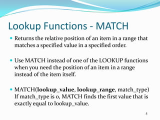
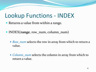
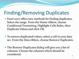
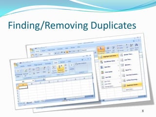
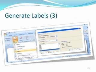
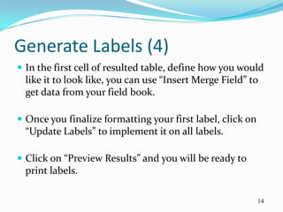
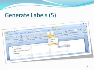
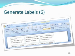
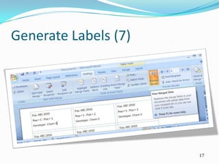
The document discusses various Excel functions for lookups, references, finding and removing duplicates, and data validation. It also provides steps for generating labels from an Excel data source using Mail Merge in Microsoft Word. Key functions covered include VLOOKUP, HLOOKUP, MATCH, INDEX, and data validation tools. Instructions are given for highlighting duplicate values, removing duplicates, and defining data validation rules. The mail merge process for linking an Excel data set to Word labels is outlined in multiple steps.

1. By Khaled Al-Shamaa

2. Relative & Absolute References
 Absolute ranges have a $ character before the column
portion of the reference and/or the row portion of the
reference.
 The $ character indicates to Excel that it should not
increment the column and/or row reference as you fill
a range with a formula or as you copy a range.
 For example A1 is a relative range, while $A$1 is an
absolute range.
2

3. Lookup Functions - VLOOKUP
 Searches for a value in the first column of a table array
and returns a value in the same row from another
column in the table array.
 VLOOKUP(value, range, column, type)
 Value: the value to search in the first column of the range.
 Range: two or more columns of data.
 Column: the column number in the range from which the
matching value must be returned.
 Type: If TRUE or omitted, an exact or approximate match
is returned. If FALSE, will only find an exact match.
3

4. Lookup Functions - HLOOKUP
 Searches for a value in the top row of a range of values,
and then returns a value in the same column from a
row you specify in the range.
 Use HLOOKUP when your comparison values are
located in a row across the top of a table of data, and
you want to look down a specified number of rows.
 Use VLOOKUP if your comparison values are located
in a column to the left of the data you want to find.
4

5. Lookup Functions - MATCH
 Returns the relative position of an item in a range that
matches a specified value in a specified order.
 Use MATCH instead of one of the LOOKUP functions
when you need the position of an item in a range
instead of the item itself.
 MATCH(lookup_value, lookup_range, match_type)
If match_type is 0, MATCH finds the first value that is
exactly equal to lookup_value.
5

6. Lookup Functions - INDEX
 Returns a value from within a range.
 INDEX(range, row_num, column_num)
 Row_num selects the row in array from which to return a
value.
 Column_num selects the column in array from which to
return a value.
6

7. Finding/Removing Duplicates
 Excel 2007 offers new methods for finding duplicates.
Select the range. From the Home ribbon, choose
Conditional Formatting, Highlight Cells Rules, then
Duplicate Values and click OK.
 To remove duplicated values, select a cell in your data
set. From the Data ribbon, choose Remove Duplicates.
 The Remove Duplicates dialog will give you a list of
columns. Choose the columns which should be
considered. 7

8. Finding/Removing Duplicates
8

9. Data Validation (1)
 Ensuring valid data entry is an important task.
 You may want to restrict data entry to a certain range of
dates, limit choices by using a list, or make sure that only
positive whole numbers are entered.
 Select one or more cells to validate. On the Data tab, click
Data Validation. The Data Validation dialog box displayed.
 Click the Settings tab and specify the type of validation
that you want.
9

10. Data Validation (2)
10

11. Generate Labels (1)
 Save and close your Excel field book, then go and open
Microsoft Word!
 Go to Mailings tab, Select Recipients, then “Use
Existing Lists…” item where you have to browse to your
Excel field book, you have to select related sheet.
 Once you define source of your data, click “Labels…”
item in “Start Mail Merge”, then select your label
vendor and type (even you can define custom one).
11

12. Generate Labels (2)
12

13. Generate Labels (3)
13

14. Generate Labels (4)
 In the first cell of resulted table, define how you would
like it to look like, you can use “Insert Merge Field” to
get data from your field book.
 Once you finalize formatting your first label, click on
“Update Labels” to implement it on all labels.
 Click on “Preview Results” and you will be ready to
print labels.
14

15. Generate Labels (5)
15

16. Generate Labels (6)
16

17. Generate Labels (7)
17

18. Thank You
18
18