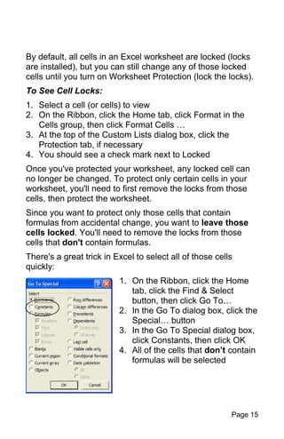
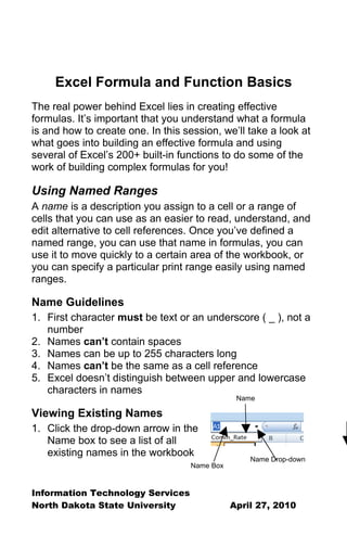
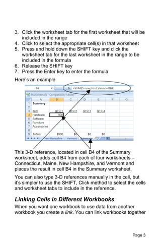
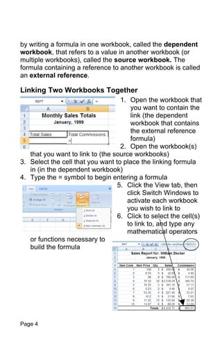
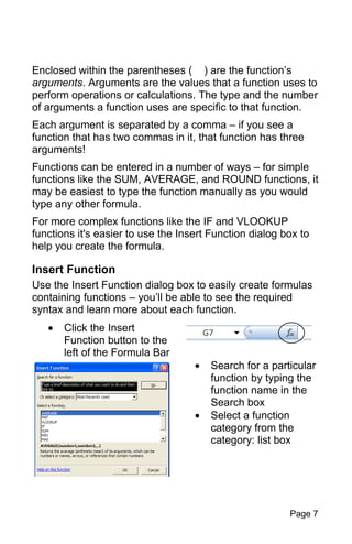
Contemporary philippine arts from the regions_PPT_Module_12 [Autosaved] (1).pptx
Â
Excel Formula and Function Basics
1. Excel Formula and Function Basics
The real power behind Excel lies in creating effective
formulas. It’s important that you understand what a formula
is and how to create one. In this session, we’ll take a look at
what goes into building an effective formula and using
several of Excel’s 200+ built-in functions to do some of the
work of building complex formulas for you!
Using Named Ranges
A name is a description you assign to a cell or a range of
cells that you can use as an easier to read, understand, and
edit alternative to cell references. Once you’ve defined a
named range, you can use that name in formulas, you can
use it to move quickly to a certain area of the workbook, or
you can specify a particular print range easily using named
ranges.
Name Guidelines
1. First character must be text or an underscore ( _ ), not a
number
2. Names can’t contain spaces
3. Names can be up to 255 characters long
4. Names can’t be the same as a cell reference
5. Excel doesn’t distinguish between upper and lowercase
characters in names
Name
Viewing Existing Names
1. Click the drop-down arrow in the
Name box to see a list of all
existing names in the workbook
Name Drop-down
Name Box
Information Technology Services
North Dakota State University April 27, 2010
2. 2. Click a name to quickly select the cell or cells within that
named range
Two Ways To Create Named Ranges:
1. Select the cell or cells to be named
2. On the Ribbon, click the Formulas tab, then click Define
Name
3. In the New Name dialog box, type a name for the range,
choose Workbook, or Worksheet from the Scope: drop-
down list, then click OK
OR:
1. Select the cell or cells to be
named
2. Click inside the Name box to
select (highlight) the current cell
address
3. Type a name for the range, then
press the Enter key
3-D References in Formulas
When you have workbooks that contain data on multiple
worksheets, you may need to use a 3-D reference to link the
data in different worksheets together in a formula so that
changes to specific cells in one worksheet will be reflected in
specific cells in another sheet.
A three-dimensional (3-D) reference is a range that spans
two or more worksheets in a workbook, linking the sheets
together.
Creating a 3-D Reference:
1. Select the cell which will contain the formula
2. Enter a formula up to the opening parenthesis i.e. =SUM(
Page 2
3. 3. Click the worksheet tab for the first worksheet that will be
included in the range
4. Click to select the appropriate cell(s) in that worksheet
5. Press and hold down the SHIFT key and click the
worksheet tab for the last worksheet in the range to be
included in the formula
6. Release the SHIFT key
7. Press the Enter key to enter the formula
Here’s an example:
This 3-D reference, located in cell B4 of the Summary
worksheet, adds cell B4 from each of four worksheets –
Connecticut, Maine, New Hampshire, and Vermont and
places the result in cell B4 in the Summary worksheet.
You can also type 3-D references manually in the cell, but
it’s simpler to use the SHIFT, Click method to select the cells
and worksheet tabs to include in the reference.
Linking Cells in Different Workbooks
When you want one workbook to use data from another
workbook you create a link. You can link workbooks together
Page 3
4. by writing a formula in one workbook, called the dependent
workbook, that refers to a value in another workbook (or
multiple workbooks), called the source workbook. The
formula containing a reference to another workbook is called
an external reference.
Linking Two Workbooks Together
1. Open the workbook that
you want to contain the
link (the dependent
workbook that contains
the external reference
formula)
2. Open the workbook(s)
that you want to link to (the source workbooks)
3. Select the cell that you want to place the linking formula
in (in the dependent workbook)
4. Type the = symbol to begin entering a formula
5. Click the View tab, then
click Switch Windows to
activate each workbook
you wish to link to
6. Click to select the cell(s)
to link to, and type any
mathematical operators
or functions necessary to
build the formula
Page 4
5. 7. Press the Enter key to enter the formula into the
dependent workbook
Here’s an example of an external reference that links three
workbooks:
This formula adds the values in cell E15 of the Decker.xls,
Simpson.xls, and Finch.xls workbooks and places the result
in a cell in the dependent workbook.
You can type these linking formulas manually, but if you use
the mouse to activate the appropriate workbooks, and select
the appropriate cells, you have less chance of making an
error in the formula’s syntax.
Once you’ve built one 3-D reference formula, or one external
reference linking formula in a workbook, you can copy those
formulas to other cells, just as you would copy any other
formula, making the job of creating multiple formulas much
easier!
Editing Links
You may need to edit the links to the source workbooks
when you’ve created an external reference formula for many
reasons. For example, you may no longer have access to a
source workbook, or you may need to link to a different
source workbook.
To Change Source Workbooks
1. Open the dependent workbook (the workbook that
contains the linking formula)
2. On the Ribbon, Click the Data tab, then click Edit Links
Page 5
6. 3. In the Edit Links dialog box, select the link you wish to
change, then click the Change Source button
4. Select the workbook you want to redirect the link to in the
Change Source dialog box, then click OK to return to the
Edit Links dialog box
5. Click Close to close the Edit Links dialog box
To Break A Link
1. Open the dependent workbook
2. On the Ribbon, click the Data tab, then click Edit Links
3. In the Edit Links dialog box, select the link you wish to
break, then click the Break Link button
4. Click Break Links in the message box that appears
5. Click Close to close the Edit Links dialog box
If you open a workbook file, and the Edit, Links command is
"grayed out" (unavailable), you are looking at a source
workbook rather than the dependent workbook. You must
open the dependent workbook to edit the links.
Excel’s Functions
Excel ships with over 200 built-in functions that can help you
create more complex formulas. You may never use most of
Excel’s functions, but you will want to be familiar with the
basic functions we’ll cover here.
Function Syntax
Each function has a particular syntax you must follow when
using that function in a formula:
=FunctionName(Argument1, Argument2, ArgumentN…)
Since functions are formulas, the first thing you need is the
equal symbol ( = ), followed by the function name.
Page 6
7. Enclosed within the parentheses ( ) are the function’s
arguments. Arguments are the values that a function uses to
perform operations or calculations. The type and the number
of arguments a function uses are specific to that function.
Each argument is separated by a comma – if you see a
function that has two commas in it, that function has three
arguments!
Functions can be entered in a number of ways – for simple
functions like the SUM, AVERAGE, and ROUND functions, it
may be easiest to type the function manually as you would
type any other formula.
For more complex functions like the IF and VLOOKUP
functions it's easier to use the Insert Function dialog box to
help you create the formula.
Insert Function
Use the Insert Function dialog box to easily create formulas
containing functions – you’ll be able to see the required
syntax and learn more about each function.
• Click the Insert
Function button to the
left of the Formula Bar
• Search for a particular
function by typing the
function name in the
Search box
• Select a function
category from the
category: list box
Page 7
8. • Click a function to select it under "Select a function:"
• The syntax for the selected function and a description
appears at the bottom of the dialog box
• To learn more about each function, select it from the
list, then click “Help on this function”
After selecting the function you want to use, click OK to
create the formula in the Function Arguments dialog box –
arguments listed in bold are required arguments; unbolded
arguments are optional and may be left empty if you don't
need them:
SUM
=SUM(Num1:NumN) [Num1:NumN indicates a range of
cells to be summed]
Replaces =A1+B1+B2, etc.
Example: =SUM(A1:B26) sums all of the values in cells A1
to A26 and B1 to B26
AVERAGE
=AVERAGE(Num1,Num2,…)
Replaces =A1+A2+A3+A4/4, etc.
Page 8
9. Example: =AVERAGE(B5:B8,D5:D7) produces the average
of all the values from B5 to B8 (argument 1) and from D5 to
D7 (argument 2) – you can use as many arguments as
necessary in the Average function
Date and Time Functions
=NOW() inserts the current system date and time into the
cell – updates whenever the worksheet is recalculated (no
arguments are required – but you still need to include the
parentheses)
=TODAY() inserts the current date without the time –
updates whenever the worksheet recalculates
Example: =TODAY()+30 calculates a date 30 days from the
current date
ROUND
=ROUND(Num, NumOfDigits)
Rounds the value specified in the first argument to the
number of digits specified in the second argument
Example: =ROUND(A6,2) A6 is the value to be rounded
(argument 1), 2 is the number of digits to round to
(argument 2).
6.555313 entered in cell A6 becomes 6.56 in the cell
containing the Round function
Decision Making Functions
The IF Function
If you learn and understand how to use only one function in
Excel, it should be the IF function.
The IF function is a very powerful decision-making function
that is often the solution to many problems in Excel.
Page 9
10. IF allows a formula to return one result if a certain condition
you specify is true, and a different result if the condition is
false. The IF function has three required arguments in this
syntax:
=IF(Logical_Test, TrueValue, FalseValue)
• The first argument – Logical_Test – is the value you are
testing. This value can be an expression (i.e. A6=6,
A2+B6>B26, etc.), or it can be another function nested
inside the IF function (AVERAGE(B6:B30)>100). The test
value must meet a condition that can be evaluated to
either True or False.
• The second argument – TrueValue – is the result you
want the formula to “return” to the cell if the evaluation of
the first argument (Logical_Test) is TRUE – this value
can be an expression, a constant value, text, or another
function nested inside the first function.
• The third argument – FalseValue – is the result you want
the formula to “return” to the cell if the evaluation of the
first argument (Logical_Test) is FALSE – this value can
also be an expression, a constant value, text, or another
function nested inside the first function.
In this example, the formula in cell F6 calculates a
commission for
the salesperson
by multiplying
the Total Sales
in cell E6 by the
18%
Commission
Rate in cell J3,
even if they
Page 10
11. didn’t meet the Quota in cell J4 (Comm_Rate is a named
range referring to cell J3, Quota refers to cell J4). The
named ranges make the formulas easier to understand and
to update.
You can add the IF function to this formula to make it
calculate a commission for each salesperson only when they
meet or exceed the quota.
The modified formula using the IF function works like this:
E6>=Quota is
the logical test
argument – if E6
is greater than or
equal to the
Quota (60,000),
then the test is
TRUE and the
result of the calculation or the value in the second argument
– E6*Comm_Rate (18%) – is returned to the cell. The third
argument is ignored.
If E6 is NOT greater than or equal to the Quota (60,000),
then the test in the first argument is FALSE and the result of
the calculation or the value in the third argument – 0 in this
case – is returned to the cell. The second argument is
ignored.
Notice the $0.00 values returned to cells F7, F9, and F10 – a
commission was not calculated for these salespeople, since
they did not meet the $60,000 quota.
If you want a formula or function to return a string of text
(characters) to a cell, enclose the text in the formula within
quote marks, like this: “No Commission”. If you wish to have
a function return a blank value (not zero) to the cell, use
Page 11
12. quote marks without a space between them. Here’s an
example:
=IF(E6>=Quota,E6*Comm_Rate,"") This formula
calculates, or returns, a commission value to the cell
containing the formula if the test is true. If the test is false, it
returns an empty string (a blank value) to that cell.
The VLOOKUP Function
The IF function allows a formula to return only two different
results – the logical test evaluates to either TRUE or FALSE.
There are many circumstances where you need your formula
to make more than one decision. This is where the
VLOOKUP function comes in handy.
The VLOOKUP function finds a value you specify in one row
and column of a lookup table that you create in another part
of your worksheet or workbook and returns a value from a
second column in the matching row of the lookup table.
This lookup table contains an orderly arrangement of
information – values in the lookup table should be sorted in
ascending order from top to bottom and the lookup table
should be placed in another part of the worksheet away from
the main body of your worksheet, or in a separate worksheet
within the workbook.
Here's the syntax of the VLOOKUP function:
=VLOOKUP(Lookup_Value,Table_Array,Col_Index_num,
Range_Lookup) – only the first three arguments are
required, the 4th argument is optional.
• Lookup_Value is the value that Excel looks up in the first
column of your lookup table. It can be a value, a cell
reference, an expression, or a text string.
Page 12
13. • Table_Array is a reference to (or the name of a reference
to) the location of your lookup table (i.e. H6:I10, or
Grades).
• Col_Index_num is the column number in the lookup table
of the column you want the value returned from (index
numbers are 1, 2, etc. from left to right rather than
column references – A, C, etc.).
• Range_Lookup is an optional argument that specifies
whether you require an exact match to the value you're
looking up, or an approximate match. If you omit this
optional argument, the VLOOKUP function uses an
approximate match which is the most appropriate in most
cases.
If you've allowed VLOOKUP to use approximate matches,
when the function can't find an exact match for the
Lookup_Value argument in the first column of the lookup
table, it uses the largest value in that column that is still less
than Lookup_Value.
Here's an example:
Lookup Table
The VLOOKUP function in this example returns a letter
grade for each student by looking up the Average value
computed in cell D2 in column 1 of the lookup table and
Page 13
14. returning the correct letter grade for the value that is less
than or equal to that value from the same row in the second
column of the lookup table.
• The first argument – D2 (Lookup_Value) tells Excel to
lookup the value in cell D2 in the lookup table.
• The second argument - $H$6:$I$10 (Table_Array) tells
the VLOOKUP function where the lookup table is stored,
the function looks in the first column of this lookup table
for an approximate match to Lookup_Value.
• The third argument – 2 (Col_Index_num) tells the
VLOOKUP function to return the value to the cell from the
second column of the lookup table from the row that
matches the approximate Lookup_Value.
• The optional fourth argument – Range_Lookup was not
used in this example.
If you change any of the values that result in the
Lookup_Value used in the VLOOKUP function being
changed, the value returned by the VLOOKUP function in
the formula will also change.
Protecting Your Worksheets
When you've spent considerable time and effort creating
complex formulas in your worksheets, you certainly don't
want to accidentally change the formula!
If you don't protect portions of your worksheets, it's very
easy to accidentally overwrite a formula with a value simply
by selecting the cell containing the formula, typing in a value,
then saving the workbook – your formula is gone!
Page 14
15. By default, all cells in an Excel worksheet are locked (locks
are installed), but you can still change any of those locked
cells until you turn on Worksheet Protection (lock the locks).
To See Cell Locks:
1. Select a cell (or cells) to view
2. On the Ribbon, click the Home tab, click Format in the
Cells group, then click Format Cells …
3. At the top of the Custom Lists dialog box, click the
Protection tab, if necessary
4. You should see a check mark next to Locked
Once you've protected your worksheet, any locked cell can
no longer be changed. To protect only certain cells in your
worksheet, you'll need to first remove the locks from those
cells, then protect the worksheet.
Since you want to protect only those cells that contain
formulas from accidental change, you want to leave those
cells locked. You'll need to remove the locks from those
cells that don't contain formulas.
There's a great trick in Excel to select all of those cells
quickly:
1. On the Ribbon, click the Home
tab, click the Find & Select
button, then click Go To…
2. In the Go To dialog box, click the
Special… button
3. In the Go To Special dialog box,
click Constants, then click OK
4. All of the cells that don’t contain
formulas will be selected
Page 15
16. To Unlock Cells:
1. With the appropriate cells selected, click the Home tab on
the ribbon, click Format in the Cells group, then click
Format Cells …
2. Click the Protection tab, if necessary
3. Remove the check mark next to Locked, then click OK
To Protect the Worksheet:
1. After unlocking the desired cells, click the Home tab, click
Format in the Cells group, then click Protect Sheet …
2. In the Protect Sheet dialog box, type a password (not
recommended) if you wish to require users to type a
password before they can remove worksheet protection,
then click OK
Once you've protected the worksheet in this manner, you
can't make any changes to any locked cells. Unlocked cells
can be changed in the normal manner.
If you need to make later changes to
the formulas inside locked cells you'll
need to remove worksheet protection,
make the changes, then reapply
worksheet protection again.
When your worksheets are protected
some of your Menu choices and
Ribbon buttons will not be available
and will appear "grayed out".
To reactivate those unavailable
options, you'll also need to unprotect
the worksheet before you can make
those changes.
Page 16
17. To Unprotect the Worksheet:
Click the Home tab, if necessary, click Format in the Cells
group, then click Unprotect Sheet …
Now that you've learned how to create formulas, and how to
use some of Excel's built-in functions, you'll be able to use
Excel to produce the results you need!
Page 17