Microsoft Excel 365 Formulas BarCharts QuickStudy 1st Edition Curtis Frye
1.
Quick and EasyEbook Downloads – Start Now at ebookmeta.com for Instant Access
Microsoft Excel 365 Formulas BarCharts QuickStudy
1st Edition Curtis Frye
https://ebookmeta.com/product/microsoft-excel-365-formulas-
barcharts-quickstudy-1st-edition-curtis-frye/
OR CLICK BUTTON
DOWLOAD EBOOK
Instantly Access and Download Textbook at https://ebookmeta.com
2.
Excel365FORMULAS
When you storedata in a workbook, you can create valuable summaries that turn your
raw data into useful information. Before we examine the mechanics of creating formulas,
here are some formula-related terms you will encounter throughout this guide:
• Formula: A statement that calculates a value in a worksheet cell.
• Function: A built-in calculation that combines values in a specific way, such as by
finding the sum of all values in a cell range.
• Argument: A value used in a formula (also the input).
• Output: The result of a formula.
• Returns: A verb describing the act of a formula generating a result, or output.
EX: The formula =3+4 returns an output of 7.
• Syntax: The structure of a function, specifying the number and order of arguments
(inputs) it requires to return a result.
Order of Operations
ExcelforOffice365follows
mathematical conventions
when determining the order
of operations used in a
calculation. That order is as
follows:
1. Parentheses: ( )
2. Negation, such as: –7
3. Percentage: %
4. Exponentiation: ^; e.g., 33
is written as 3^3
5. Multiplication and division: * and /
6. Addition and subtraction: + and –
EX: 4 + 8 * 7 = 60, where 8 * 7 = 56, and 4 + 56 = 60.
If two operations on the same level, such as multiplication and division, occur outside
parentheses, Excel performs them in left-to-right order.
EX: 8 * 5/4 = 10. You can change the order of operations by using parentheses.
EX: (4 + 8) * 7 = 84, where 4 + 8 = 12, and 12 * 7 = 84.
Creating Formulas
Create a formula:
Type an equal sign (=) followed by the values, cell references,
or functions to be used in the calculation.
NOTE: The first character in a cell containing a formula must
be =. If it is any other character, including a space, Excel
interprets the cell’s contents as text.
Refer to cells & cell ranges in formulas:
• Worksheet cells are identified by their column letter and
then their row number.
• The top-left cell in a worksheet is in column A and row 1,
so its cell address is A1.
• You can also refer to cell ranges, or collections of cells.
• To identify a cell range, type the address of the cell at the top-
left corner of the range, followed by a colon, and then the cell
at the bottom-right corner of the range.
EX: The reference for cells 6 through 10 in columns A and B
would be A6:B10.
• To create a reference to multiple, noncontiguous groups of
cells, put a comma between the references.
EX: Finding the sum of the values in the cell range A1:B5
and the range F1:G5 would call for the formula =SUM(A1:B5,
F1:G5).
Create relative, absolute & mixed references:
• When you type a cell reference with just the column letter and
row number, such as A1, that reference can change when you
copy its formula to another cell.
EX: Copying the formula =A1 + A2 and pasting it one cell to
the right would create the formula =B1 + B2. The destination
cell is one column to the right of the original cell, so Excel
changes the formula’s references based on that difference.
• To create an absolute reference, one that doesn’t change when
you copy a formula, type a dollar sign ($) before the column
and row designators.
EX: The formula =$A$1 * $A$2 won’t change regardless of
the cell you paste it into.
• You can also create a mixed reference, where either rows or
columns are absolute, by adding $ before just the element
you want to remain the same.
EX: The cell reference A$1 allows changing columns and
$A1 allows changing rows.
Insert a function:
• Start creating the formula where you want to insert the
function, and then do one of the following:
- Type the first letters of the function name, and either finish
typing its name, or click the function on the AutoComplete
list that appears and press <Tab>.
- Click the Insert Function button and select the
function you want to add.
- Go to the Function Library group on the Formulas tab,
click the category of the function you want to add, and then
click the function name.
Get help using function argument ToolTips:
• Start creating a formula, and enter the name of the function
followed by a left parenthesis, such as =SUM(.
• In the function ToolTip that appears below the cell that
contains the formula, position the mouse pointer over the
function name.
• When the function name’s text changes to a blue, underlined
format, click it to display the relevant help file.
Using Tables in Formulas
Tables give formal structure to lists of data in a worksheet, with
unique names for the table as a whole and for each column.
EX: A table named Table1 (the default name for the first
table you create in a workbook) could have columns
named Date, StoreNumber, and Sales.
You could summarize the table’s data using formulas,
PivotTables, or charts. When you create tables, Excel
automatically updates your formulas, PivotTables, or charts
when you add a row of data. If you add data to a worksheet
outside a table, you must edit the summary’s settings to reflect
the new values.
Create a table:
• Click any cell in a data list.
• Go to the Styles group on the Home tab.
• Click Format as Table.
• In the gallery that appears, click the style you want to apply.
• In the Format As Table dialog box, verify that Excel has
identified the correct cell range, check the My table has
headers box if appropriate, and click OK.
Refer to a table column in a formula:
• Start creating a formula in a cell, such as
=AVERAGE().
• In the parentheses, type the name of the table or start
typing it and select it from the suggestions list.
• Type a left square bracket ([), click the name of the
column you want to summarize, and then type a right
square bracket (]): = AVERAGE(Sales16[Sales]).
• Finish editing your formula and press <Enter>.
Add an AutoSum function:
• Select a cell below a column of numbers.
• Go to the Editing group on the Home tab.
• Click the AutoSum button
to add a SUM formula, or click the AutoSum
button’s down arrow to select another function.
TIP: To add an AutoSum formula that uses
the SUM function, select the cell and press
<Alt> + <=>.
Create a link to a cell or cell range
not on the current worksheet:
• If necessary, open the workbook that contains
the outside data you want to use in your
formula.
• Start creating the formula where you want
to use data in cells in another worksheet or
workbook.
• Display the external worksheet, and then select
the cells that contain the data to include in the
formula.
• Finish entering the formula, and press
<Enter>.
NOTE: Excel follows worksheet names with an
exclamation point (e.g., CashFlow!$E$4) and
encloses workbook names in square brackets
(e.g., [FinanceCheck]CashFlow!$E$4). If
the workbook or worksheet name contains
a space, Excel puts single quotes around the
workbook and worksheet references (e.g.,
‘Cash Flow’!$E$4).
1
WORLD’S #1 QUICK REFERENCE SOFTWARE GUIDE
3.
Organizing Data UsingNamed Ranges
Define a named range using the
Name box:
• Select the cells you want to be part of the
named range.
• In the Name box , type the name of the
range and press <Enter>.
Define a named range using the
Name Manager:
• Go to the Defined Names on the Formulas tab.
• Click Name Manager.
• Click New.
• In the Name box, edit the name of the named
range.
• Click the Collapse Dialog button to the
right of the Refers to box, and then select the
cells in the range.
• Click the Expand Dialog button to the
right of the Refers to box.
• Click OK.
• In the Name Manager dialog box, click Close.
Create a series of named
ranges using labels as
range names:
• Select the cells that contain the
labels and values for the named
ranges.
• Go to the Defined Names group
on the Formulas tab.
• Click Create from Selection.
• In the Create Names from
Selection dialog box, check the
box or boxes indicating where
the ranges’ names are stored (e.g.,
Left column and Top row).
• Click OK.
NOTE: If your named range’s
label duplicates a cell address,
such as NE01 or another reserved
word, Excel adds an underscore
to make the name unique. For
example, NE01 becomes NE01_.
Use a named range in a
formula:
• Type an equal sign, followed by
the start of the formula, such as
=AVERAGE(.
• In place of a cell range, type the
name of the named range and then
complete the formula.
EX: =AVERAGE(Length), where
Length is the name of the named
range.
• Press <Enter>.
TIP: When you start typing
the name of a named range,
it will appear in the formula
AutoComplete list along with the
other functions that start with the
letters you’ve typed. Function
names are always displayed in
capital letters, so you should
consider using an initial capital
letter followed by lowercase letters
for named ranges to set them apart.
Edit a named range:
• Go to the Defined Names group on the Formulas
tab.
• Click Name Manager.
• Click the named range you want to edit.
• Click Edit.
• In the Name box, edit the name of the named range.
• Click the Collapse Dialog button to the right of the
Refers to box, and then select the cells in the range.
• Click the Expand Dialog button to the right of the
Refers to box.
• Click OK.
• In the Name Manager dialog box, click Close.
Delete a named range:
• Go to the Defined Names group on the Formulas
tab.
• Click Name Manager.
• Click the named range you want to edit.
• Click Delete.
• In the confirmation dialog box that appears, click
OK.
• In the Name Manager dialog box, click Close.
Summary & Statistical Functions
Spreadsheets store numerical data
efficiently, so it makes sense that
Excel includes literally hundreds
of summary and statistical
functions you can use to analyze
and summarize your data. The
functions in this section all take
values, cell ranges, or combinations
of the two as arguments.
EX: The formula =SUM(14, 15,
C8:C10) would add 14 to 15, and
then add the values in the cell range
C8:C10 to that total.
Each of the following functions
follow the same syntax,
function(number1, [number2]…).
• function: Name of the function.
• number1: Required argument
consisting either of a number or
the address of a cell or cell range
that contains numbers.
• number2 and subsequent
number arguments: Additional
ranges to be included in the
summary.
The following functions are the
most commonly used summary and
statistical functions:
• SUM: Adds the values in all
named cells.
• PRODUCT: Multiplies the values
in all named cells.
• AVERAGE: Finds the arithmetic
average, or mean, of the values in
all named cells.
• MEDIAN: Finds the middle
value in the value list when the
values are sorted into ascending
numerical order. If there is an
even number of values, the
middle two values are averaged.
• MODE.SNGL: Finds the most
common value in the set.
• MODE.MULT: Finds the most
common values in the set. To
enter a formula that uses this
function, select a range of cells
that reflect the number of values
you want to return.
EX: If you want to find the two most
common values, select two cells, and
then type in a formula such as: = MODE.
MULT($C$18:$C$C26). Press <Ctrl> +
<Shift> + <Enter> to enter the formula as
an array formula.
• MIN: Finds the minimum value in the set,
ignoring logical values and text.
• MINA: Finds the minimum value in the set,
including logical values and text.
• MAX: Finds the maximum value in the set,
ignoring logical values and text.
• MAXA: Finds the maximum value in the set,
including logical values and text.
• STDEV.P: Finds the standard deviation of
the values in the set by using all values in the
set.
• STDEV.S: Finds the standard deviation of
the values in the set by using a sample of
values from the set.
• VAR.P: Finds the variance of the values in
the set by using all values in the set.
• VAR.S: Finds the variance of the values in the
set by using a sample of values from the set.
You can also find the sum or average of values
that meet criteria you set.
EX: You could find the sum of all sales to
customers in Virginia or calculate the average
value of months with sales under $250,000
(see the table shown here).
Find the sum of data that meets
one condition:
• In a worksheet cell, create a formula of
the form =SUMIF(range, criteria, [sum_
range]), where:
- range represents the cells that contain the
values to be evaluated using the formula’s
criteria.
- criteria represents the rule used to evaluate
whether to include a value in the summary.
- sum_range is an optional argument
that identifies the cells that contain the
numerical values to be included in the
summary, if they are different from the
cells identified by the range argument.
• Press <Enter>.
• Given the sample data in the table shown in
this section, the formula =SUMIF(C2:C10,
”Virginia”, D2:D10) would return $735,691.
Find the sum of data that meets
multiple conditions:
• In a worksheet cell, create a formula of the
form =SUMIFS(sum_range, criteria_range1,
criteria1, [criteria_range2], [criteria2]…),
where:
- sum_range represents the cells that contain
the numerical values to be included in the
summary.
- criteria_range1 represents the cells that
contain the values to be evaluated using
the formula’s first criteria.
- criteria1 represents the first rule used to
evaluate whether to include a value from
criteria_range1 in the summary.
- criteria_range2 is an optional argument
that lists the cells that contain the values
to be evaluated using the formula’s second
criteria.
- criteria2 is an optional argument that
represents the second rule used to evaluate
whether to include a value from criteria_
range2 in the summary (you can create
additional criteria and criteria_range
pairs to further limit which values should
be included in the summary).
• Press <Enter>.
• Given the sample data in the table shown in
thissection,theformula=SUMIFS(D2:D10,
C2:C10,”Delaware”, B2:B10,”February”)
would return $156,634.
Find the average of data that
meets one condition:
• In a worksheet cell, create a formula of
the form =AVERAGEIF(range, criteria,
[average_range]), where:
–range represents the cells that contain
the values to be evaluated using the
formula’s criteria.
–criteria represents the rule used to
evaluate whether to include a value in the
summary.
–average_range is an optional argument
that identifies the cells that contain the
numerical values to be included in
the summary, if they are different
from the cells identified by the range
argument.
• Press <Enter>.
• Given the sample data in the table shown
in this section, the formula =AVERAGEIF
(B2:B10,”March”,D2:D10) would return
$213,233.
Find the average of data that
meets multiple conditions:
• In a worksheet cell, create a formula of
the form =AVERAGEIFS(average_range,
criteria_range1, criteria1, [criteria_range2],
[criteria2]…), where:
–average_range represents the cells
that contain the numerical values to be
included in the summary.
–criteria_range1 represents the cells that
contain the values to be evaluated using
the formula’s first criteria.
–criteria1 represents the first rule used to
evaluate whether to include a value from
criteria_range1 in the summary.
–criteria_range2 is an optional argument
that lists the cells that contain the values
to be evaluated using the formula’s
second criteria.
–criteria2 is an optional argument that
represents the second rule used to evaluate
whether to include a value from criteria_
range2 in the summary (you can create
additional criteria and criteria_range
pairs to further limit which values
should be included in the summary).
• Press <Enter>.
• Given the sample data in the table shown in
this section, the formula =AVERAGEIFS
(C2:C10,C2:C10,”<200000”,B2:B10,
”Florida”) would return $440,072.
2
4.
Counting Values inCell Ranges
In addition to summarizing values in a range using SUM,
AVERAGE, or another arithmetic function, you can count
the number of values of specific types that appear in a
range. The basic COUNT family of functions all follow
the syntax of function(value1, [value2]…), where:
• value1 is a cell reference or range.
• value2 and subsequent value arguments are optional
arguments that refer to subsequent cell ranges.
The basic COUNT functions are:
• COUNT: Counts the number of cells that contain
numbers.
• COUNTA: Counts the number of cells in a range that
are not empty.
• COUNTBLANK: Counts the number of cells in a range
that are blank.
You can also use the conditional versions of COUNT,
COUNTIF, and COUNTIFS to count values that meet
one or more criteria.
Count cells that contain data that meets
one condition:
• In a worksheet cell, create a formula of the form
=COUNTIF(range, criteria), where:
- range represents the cells that contain the values to be
evaluated using the formula’s criteria.
- criteria represents the rule used to evaluate whether to
include a value in the summary.
• Press <Enter>.
• Given the sample data in the table shown in the
Summary & Statistical Functions section, the formula
=COUNTIF(D2:D10,”<300000”) would return 7.
Count cells that contain data that meets
multiple conditions:
• In a worksheet cell, create a formula of the form
=COUNTIFS(range1, criteria1, [range2], [criteria2]…),
where:
- range1 represents the cells that contain the values to be
evaluated using the formula’s first criteria.
- criteria1 represents the rule used to evaluate whether to
include a value from range1 in the summary.
- range2 is an optional argument representing a second
set of values to be evaluated using the formula’s second
criteria.
- criteria2 is an optional argument that represents the
second rule used to evaluate whether to include a value
from range2 in the summary (you can create additional
range and criteria pairs to further limit which values
should be included in the summary).
• Press <Enter>.
• Given the sample data in the table shown in the Summary
& Statistical Functions section, the formula
=COUNTIFS(B2:B10,”February”,D2:D10,”>200000”)
would return 2.
Performing Financial Calculations
Principal & Interest Payments
Financing a private purchase or business venture requires you to
repay the loan over time. A fully amortized loan, one that is paid in
full at the end of the term, requires periodic payments that are often
made on a monthly basis. The PMT function calculates the periodic
payment required to pay off a loan over the time frame you specify.
Each payment has an interest and principal component, which can
be calculated using the IPMT and PPMT functions, respectively.
Use the PMT function:
• In a worksheet cell, create a formula of the form =PMT(rate,
nper, pv, [fv], [type])rate, where:
- rate is the annual interest rate, which should be divided by
the number of payments per year.
EX: For a loan with a 4.8% interest rate and monthly
payments, the rate would be 4.8%/12 (see table below).
- nper is the number of payments.
- pv is the present value, or principal, of the loan.
- fv is an optional argument for the future value of the loan.
Most loans are paid in full (fully amortized) at the end of the
payment period, so this value can usually be omitted.
- type is an optional argument for when the payment is due. If
omitted or 0, the payment is due at the end of the period (almost
always true); if 1, the payment is due at the start of the period.
EX: =PMT(4.8%/12, 360, 350000) returns the value –$1,836.33.
The formula returns a negative value because it represents cash
you owe.
TIP: It is common practice to multiply the PMT function’s result
by –1 to display the result as a positive number.
Use the IPMT & PPMT functions:
The IPMT and PPMT functions use the same rate, nper, pv, fv, and
type arguments along with the per argument.
• In a worksheet cell, create a formula of the form =IPMT(rate,
per, nper, pv, [fv], [type]) or =PPMT(rate, per, nper, pv, [fv],
[type]), where:
• per is the period for which you are calculating the
interest and principal components of the payment.
EX:=IPMT(4.8%/12,12,360,350000)returns–$1,380.41,
and =PPMT(4.8%/12, 12, 360, 350000) returns –$455.92.
Adding $1,380.41 + $455.92 (the absolute values of the
payment) gives you $1,836.33, which corresponds to the
result of the PMT function.
Calculating Present Value
The PV function calculates the present value of a
series of payments given the number of payments, the
amount of each payment, and the interest rate you want
to assume.
Use the PV function:
In a worksheet cell, create a formula of the form
=PV(rate, nper, pmt, [fv], [type]), where:
• rate is the annual interest rate, which should be
divided by the number of payments per year.
EX: For a loan with a 6% interest rate and monthly
payments, the rate would be 6%/12.
• nper is the number of payments.
• pmt is the amount of each payment (this value must
remain constant).
• fv is an optional argument for the future value of the
loan. Most loans are paid in full (fully amortized)
at the end of the payment period, so this value can
usually be omitted.
• type is an optional argument for when the payment is
due. If omitted or 0, the payment is due at the end of
the period (almost always true); if 1, the payment is
due at the start of the period.
EX: =PV(6%/12, 60, 1000), which calculates the present
value of 60 monthly payments of $1,000 each and
assumes a 6% annual interest rate, returns –$51.725.56.
As with the PMT function, PV returns a negative value
because it assumes the money is leaving your account.
The formula’s result is less than the nominal sum of
the payments, $60,000, because future payments are
discounted at a 6% annual rate.
Calculating Future Value
Just as the PV function calculates the present value of
a series of future payments, the FV function calculates
the future value of a payment made today.
Use the FV function:
In a worksheet cell, create a formula of the form
=FV(rate, nper, pmt, [pv], [type]), where:
• rate is the annual interest rate, which should be
divided by the number of payments per year.
EX: For a loan with a 6% interest rate and monthly
payments, the rate would be 6%/12.
• nper is the number of payments.
• pmt is the amount of each payment (this value must
remain constant). If the pmt value is 0 or omitted,
you must include a value for pv.
• pv is an optional argument for the present value of
the annuity. If the pv value is 0 or omitted, you must
include a value for pmt.
• type is an optional argument for when the payment
is due. If omitted or 0, the payment is due at the end
of the period (almost always true); if 1, the payment
is due at the start of the period.
EX: =FV(6%/12, 60, 1000), which represents the future
value of 60 monthly payments of $1,000 with an annual
interest rate of 6%, returns –$69,770.03.
EX: =FV(6%/12, 60, 0, 10000), which represents the
future value of a $10,000 payment where 6% interest
is compounded monthly over 60 months, returns
–$13,488.50.
Calculating Time to Reach an
Investment Goal
If you have a savings or investment target, you can
use the PDURATION function to calculate how long
it will take you to reach your goal.
Use the PDURATION function:
In a worksheet cell, create a formula of the form
=PDURATION(rate, pv, fv), where:
• rate is the annual interest rate, which should
be divided by the number of times interest is
compounded per year.
• pv is the present value of the investment.
• fv is the future value you want to achieve.
EX: =PDURATION(6%/12, 10000, 25000), which
calculates how long it will take a $10,000 investment
to reach $25,000, assuming 6% interest compounded
monthly, returns 183.72 months, or a little over 15
years.
3
5.
Processing Text UsingFormulas
Extracting Text From a Cell
Business operations often generate text that follows a
known pattern. For example, a university class might
have a four-letter code, such as ACCT, that indicates the
class’s academic department, followed by a three-digit
number. When your text follows a predictable pattern,
you can use the LEFT, RIGHT, and MID functions to
extract the values you want.
Use the LEFT & RIGHT functions:
LEFT returns a number of characters from the left end, or
beginning, of a text string. The RIGHT function returns
the right-most characters from the text string.
In a worksheet cell, create a formula of the form
=LEFT(text, num_chars) or =RIGHT(text, num_chars),
where:
• text is the cell that contains the text, or a text string
enclosed in double quotes.
• num_chars is the number of characters to return.
Use the MID function:
MID returns characters from the middle of a string. With
MID, you must specify the starting point in the string, the
number of characters to return, and the cell to look in.
In a worksheet cell, create a formula of the form
=MID(text, start, num_chars), where:
• text is the cell that contains the text, or a text string
enclosed in double quotes.
• start is the position of the first character in the string
that MID should return.
• num_chars is the number of characters to return.
EX: If cell G5 contains the text ACCT358L01,
=LEFT(G5, 4) returns ACCT,
=RIGHT(G5, 3) returns L01, and
=MID(G5, 5, 3) returns 358.
Use the UPPER, LOWER & PROPER functions:
Text entered into Excel, or brought in from outside sources, can take
on a variety of forms. Some text might be stored as all capital letters,
especially if it’s part of a data collection from a legacy system. You can
use the PROPER, UPPER, and LOWER functions to change the text into
the form you need. UPPER and LOWER changes text to all uppercase or
lowercase letters, respectively, whereas PROPER makes the first letter
of each word uppercase and the remaining letters lowercase.
In a worksheet cell, create a formula of the form =UPPER(text),
=LOWER(text), or =PROPER(text), where:
• text can be either the address of the cell that contains the text to analyze
or a text string enclosed in double quotes.
EX:=UPPER(“Adequateinventory.”)returns“ADEQUATEINVENTORY.”
Cleaning Imported Data
Data imported from outside sources can sometimes include characters
that Excel doesn’t handle well. These so-called nonprinting characters
can wreak havoc with your formulas and text displays. The CLEAN
function removes those unwanted characters from your data set, letting
you work with just the characters you can handle easily.
Use the CLEAN function:
In a worksheet cell, create a formula of the form =CLEAN(text), where:
• text can be either the address of the cell that contains the text to analyze
or a text string enclosed in double quotes.
Use the TRIM function:
The TRIM function makes your text data easier to work with by removing
all whitespace (e.g., tabs, spaces, and carriage returns) from a text string
except for single spaces between words.
In a worksheet cell, create a formula of the form =TRIM(text), where:
• text can be either the address of the cell that contains the text to analyze
or a text string enclosed in double quotes.
EX: =TRIM(“Adequate inventory . ”) returns “Adequate inventory.”
Combining
Multiple Text
Strings
When your worksheet has text in
several cells, you can combine
the values together using the
CONCATENATE function or the
& operator. Both methods can
add values from cells or literal
strings you type between double
quotes—which one you use
depends on the nature of your data
and your personal preference.
Use the CONCATENATE
function:
In a worksheet cell, create
a formula of the form
=CONCATENATE(text1, [text2]…),
where:
• text1 is a required argument that
contains a cell address or text
string enclosed in double quotes.
• text2 and subsequent arguments
are optional arguments that
contain additional text strings.
EX: =CONCATENATE(“19”, “ ”,
“cases”) returns 19 cases. =“35”
& “ ” & “bottles” returns 35
bottles.
Performing Conditional Calculations Using IF & IFERROR
Logical Comparisons
When you calculate values such as sales commissions, it’s likely you will want to
apply different rules to different values. For example, a salesperson might receive a
6% commission on sales up to $10,000 and 8% when total sales are over $10,000.
The IF and IFS functions let you make logical comparisons, in this case to test which
calculation to perform. The IF function works best when a single true or false logical
test is made; IFS works best if there are more than two possible outcomes.
NOTE: You can use nested IF functions to test for multiple conditions, but the IFS
function’s syntax is easier to read. The IF and IFS functions return a result as soon as
the first true condition is found.
Use the IF function:
In a worksheet cell, create a formula of the form =IF(logical_test, value_if_true,
[value_if_false]), where:
• logical_test is the statement Excel evaluates to determine which condition to follow.
• value_if_true is the value or calculation to use if the condition is met.
• value_if_false is the value or calculation to use if the condition is not met.
EX: Cell G5 contains the value 15000. The formula =IF(G5>10000, G5*8%,
G5*6%) returns 1200, which is 15000 * 8%. If cell G5 contained the value 9000,
then the formula would return 540, which is 6% of 9000.
Use the IFS function:
In a worksheet cell, create a formula of the form =IF(logical_test_1, value_if_true_1,
[logical_test_2], [value_if_true_2], …, “TRUE”, other_value), where:
• logical_test_1 is the statement Excel evaluates first.
• value_if_true_1 is the value or calculation to use if the condition is met.
• logical_test_2 (and subsequent logical tests) is the statement Excel evaluates if the
previous condition is not met.
• value_if_true_2 (and subsequent values) is the value or calculation to use if a
specific condition is met.
• “TRUE” is a default condition to apply if none of the previous conditions are
met.
• other value is the value or calculation to use if no previous conditions are met.
EX: Cell G5 contains the value 15000. The formula =IF(G5>=25000, G5*8%,
G5>=20000, G5*7%, G5>=15000, G5*6%, G5>=12500, G5*5%, “TRUE”,
G5*4%) returns 1200, which is 15000 * 8%. If cell G5 contained the value 9000,
then the formula would return 360, which is 4% of 9000.
TIP: If you have a condition where a value can either meet or not meet a single
test, use the IF function.
Error Codes
When a formula results in an error, such as when an input cell is blank or contains
text when the function expects a number, Excel displays an error code. Rather
than show the error code, you can use the IFERROR function to specify the text
that appears in a formula’s cell if the formula returns one of these error types:
#DIV/0!, #N/A, #NAME?, #NULL!, #NUM!, #REF!, and #VALUE!.
Use the IFERROR function:
In a worksheet cell, create a formula of the form =IFERROR(value, value_if_
error), where:
• value is a calculation that the IFERROR function checks for an error. If there is
no error, the IFERROR function returns the result of the calculation.
• value_if_error specifies the text the IFERROR function displays if the value
argument’s calculation returns an error.
EX: =IFERROR(14000/0, “An error occurred”) returns “An error occurred.”
Performing Date Calculations
Extracting the Day, Month,
or Year From a Date
If you know an important date, such as the day
a project is scheduled for completion, you can
use Excel functions DAY, MONTH, and YEAR
to find the named component of that date.
Use the DAY, MONTH & YEAR functions:
In a worksheet cell, create a formula of the form =DAY(date),
MONTH(date), or YEAR(date), where:
• date is a date, such as 8/2/2021, or a serial number that represents
a date. Excel tracks dates using whole numbers counted from
1/1/1900, so 8/2/2021 is day 44,410. Time is saved as the decimal
component of the number, so 44410.5 would be noon on 8/2/2021.
EX: If cell A3 contains the date 11/16/21, then
=DAY(A3) returns 116.
Use the WEEKDAY function:
The WEEKDAY function tells you the weekday
on which a particular date falls.The default return
values are for Sunday to be day 1 and Saturday to
be day 7, but you can change those values.
4
6.
Performing Date Calculations(continued)
Finding & Displaying Cell Values & Formula Text
Look Up Cell Values
One of the benefits of Excel’s grid layout is the ability to create lists of
information and use formulas to look up values based on other information.
Using the data list shown here in the table, you could use the VLOOKUP
function to search for a product’s name based on a known ProductID value.
The VLOOKUP function requires your lookup value to appear in the left-
most column of the lookup table. The new XLOOKUP function is much
more flexible and lets you base the lookup operation on values in any column
of the lookup array.
Use the VLOOKUP function:
In a worksheet cell, create a formula of the form =VLOOKUP(lookup_value,
table_array, col_index_num, [range_lookup]), where:
• lookup_value is a value or, usually, address of the cell that contains the
value to be found in the first table column.
• table_array is the cell range that contains the values to be considered part
of the table.
• col_index_num is the table column that contains the value to be returned by
the formula.
• [range_lookup] is an optional argument specifying whether the formula
allows an approximate match (TRUE or blank) or requires an exact match
(FALSE). If this argument is set to FALSE, any value greater than the last
value in the left-most column returns a result from the last row. If the
lookup_value is less than the first value in the left-most column, or if an
exact match isn’t found when required, the formula returns an #N/A error.
EX: Using the data in the table, the formula =VLOOKUP(G12,G6:I10,2,
TRUE) returns “Yellow beach ball.”
Use the XLOOKUP function:
In a worksheet cell, create a formula of the form =XLOOKUP(lookup_value, lookup_
array, return_array, [range_lookup]), where:
• lookup_value is a value or, usually, address of the cell that contains the value to be found
in the first table column.
• lookup_array is the cell range that contains the values to be considered part of the table.
• return_array is the cell range that contains the value to be returned by the formula.
• [if_not_found] is an optional argument specifying what the formula should display if it
cannot return a result. If the formula cannot return a result and if_not_found is blank, the
formula returns an #N/A error.
• [match_mode] is an optional argument specifying how XLOOKUP should return a
match or near match. The default condition is to look for an exact match and return
either an #N/A error or the value of the [if_not_found] argument if there is none, but you
can specify whether to return the next smallest item, next largest item, or an item that
meets a wildcard criterion.
• [search_mode] is an optional argument specifying how XLOOKUP should search
within the lookup_array. The default method is to search from the top down and return
the appropriate value from the return_array, but you can specify whether to search from
the bottom up, perform a binary search on a list sorted into ascending order, or perform
a binary search on a list sorted into descending order.
EX: Using the data in the table, the formula =XLOOKUP(“Blue
cooler”,H6:H10,I6:I10,”Not found”) returns 24.99, while =XLOOKUP(“Red
cooler”,H6:H10,I6:I10,”Not found”) returns “Not found” because there is no exact
match for Red cooler.
Display Formula Text
Excel gives you the ability to create sophisticated formulas, but it can be difficult for
your colleagues to understand how a formula works without seeing it in its entirety. You
can always click the cell and look at both the result in the cell and the formula on the
formula bar, but it’s easy to lose your place when you switch between the two places in
the program window. The FORMULATEXT function displays the text of a formula from
one worksheet cell in another cell.
Use the FORMULATEXT function:
In a worksheet cell, create a formula of the form =FORMULATEXT(reference), where:
• reference is the address of the cell that contains the formula you want to display.
EX: If cell H12 contains the formula =VLOOKUP(G12,G6:I10,2,TRUE), then
=FORMULATEXT(H12) returns =VLOOKUP(G12,G6:I10,2,TRUE).
Division, Decimals & Rounding
Dividing Values to Find
Quotients & Remainders
Many businesses sell items by the case, where
each case contains a set number of items. For
example, a case of olive oil could hold a dozen
bottles. When you know how many individual
items you have on hand, you can calculate how
many full cases you can make from those items.
Use the QUOTIENT function:
The QUOTIENT function does the calculation
by dividing one number by another and
discarding the remainder.
In a worksheet cell, create a formula of the
form =QUOTIENT(numerator, denominator),
where:
• numerator is the value to be divided.
• denominator is the value by which the other
arguments are divided.
Use the MOD function:
The MOD function performs the complementary
calculation, dividing one number by another and
returning the remainder. You could use MOD to
find out how many items you would have left
over if you have 53 bottles of olive oil sold in
cases of 12 bottles.
In a worksheet cell, create a formula of the form
=MOD(number, divisor), where:
• number is the value to be divided.
• divisor is the value by which the other
arguments are divided.
Finding the Integer &
Decimal Parts of Numbers
Just as the QUOTIENT and MOD functions
return the quotient and remainder of a division
operation, the INT function returns the integer
portion of a number.
Use the INT function:
You can use INT to find the decimal part of the number by subtracting
the result of the INT function from the number itself.
In a worksheet cell, create a formula of the form =INT(number),
where:
• number is a numerical value or address of a cell that contains a
numerical value.
EX: =INT(14.8) returns 14.
=14.8 – INT(14.8) returns 0.8.
Rounding Numbers Up & Down
Businesses like to deal in whole numbers, whether managing hours of
work or the number of products you need to produce to meet projected
demand. For example, if you can make only 10 units of a product at
a time, you will need to make 50 units to meet a demand of 41 units.
There are three functions that round numbers up or down.
ROUND takes two arguments: the number to be rounded and the
number of digits to the right of the decimal point to which the
number should be rounded.
In a worksheet cell, create a formula of the form
=WEEKDAY(date, [return_type]), where:
• date is the cell address or serial number of the
date.
• return_type, an optional argument used with
the WEEKDAY function, lets you specify the
counting system and first day of the week. If the
argument is left blank or set to 1, then Sunday
is day 1 and Saturday is day 7. If return_type is
set to 2, then Monday is day 1 and Sunday is day
7. The other options, which are used much less
frequently, appear in the formula AutoComplete
list when you create the formula.
Calculating the Days
Between Dates
Businesses often need to know the number of days
between two dates. For example, if you know the
start date and end date of a project, you can use
Excel to calculate the number of days, months, or
years between those dates. If you want to find the
number of days between two dates, you can use the
DATEDIF function.
NOTE: Microsoft hasn’t documented DATEDIF,
and no ToolTip, AutoComplete, or other information
about the function appears in the help system.
Use the DATEDIF function:
In a worksheet cell, create a formula of the form
=DATEDIF(date1, date2, interval), where:
• date1 is the cell address or serial number of the earlier date.
• date2 is the cell address or serial number of the later date.
• interval is the type of difference you want to calculate.
- “d” calculates the number of days.
- “m” calculates the number of months.
- “y” calculates the number of years.
NOTE: Partial months and years are rounded down, so a
difference of 9 months and 23 days would return a value of 9.
EX: If C16 contains 7/1/21 and C15 contains 7/15/21, then
=DATEDIF(C16, C15, “d”) returns 14.
5
bring them tothe touch, without trusting to their glitter or their
sound;—so, to recognise good people and persons of virtue, it is
needful to observe the splendour of their deeds, without dwelling
upon their mere talk.”[100]
The narrative which Paradin neglects to give may be supplied from
other sources. This Emblem or Symbol is, in fact, that which was
appropriated to Francis I. and Francis II., kings of France from 1515 to
1560, and also to one of the Henries—probably Henry IV. The
inscription on the coin, according to Paradin and Whitney’s woodcut, is
“Franciscvs Dei Gratia Fran. Rex;” this is for Francis I.; but in the
Hierographia Regvm Francorvm[101]
(vol. i. pp. 87 and 88), the emblem
is inscribed, “Franciscus II. Valesius Rex Francorum XXV.
Christianissimus.” A device similar to Paradin’s then follows, and the
comment, Coronatum aureum nummum, ad Lydium lapidem dextra
hæc explicat & sic, id est, duris in rebus fidem explorandam docet,
—“This right hand extends to the Lydian stone a coin of gold which is
wreathed around, and so teaches that fidelity in times of difficulty is
put to the proof.” The coin applied to the touchstone bears the
inscription, “Franciscvs II. Francorv. Rex.” An original drawing,[102]
by
Crispin de Passe, in the possession of Sir William Stirling Maxwell,
Bart., of Keir, presents the inscription in another form, “Henricvs, D. G.
Francorv. Rex.” The first work of Crispin de Passe is dated 1589, and
Henry IV. was recognised king of France in 1593. His portrait, and that
of his queen, Mary of Medicis, were painted by De Passe; and so the
Henry on the coin in the drawing above alluded to was Henry of
Navarre.
The whole number of original drawings at Keir, by Crispin de Passe, is
thirty-five, of the size of the following plate,—No 27 of the series.
10.
Crispin de Passe,about 1595.[103]
The mottoes in Emblemata Selectiora are,—
“Pecunia sanguis et anima mortalium.
Quidquid habet mundus, regina Pecunia vincit,
Fulmineoque ictu fortius una ferit.”
“’t Geld vermag alles.
’t Geld houd den krygsknecht in zyn plichten,
Kan meer dan’t dondertuig uit richten.”
“Money the blood and life of men.
Whatever the world possesses, money rules as queen,
And more strongly than by lightning’s force smites together.”
“Money can do everything.
To his duty the warrior, ’tis money can hold,—
Than the thunderbolt greater the influence of gold.”
11.
Very singular isthe correspondence of the last two mottoes to a scene
in Timon of Athens (act iv. sc. 3, lines 25, 377, vol. vii. pp. 269, 283).
Timon digging in the wood finds gold, and asks,—
“What is here?
Gold! yellow, glittering, precious gold!”
and afterwards, when looking on the gold, he thus addresses it,—
“O thou sweet king-killer, and dear divorce
’Twixt natural son and sire! thou bright defiler
Of Hymen’s purest bed! thou valiant Mars!
Thou ever young, fresh, loved, and delicate wooer,
Whose blush doth thaw the consecrated snow
That lies on Dian’s lap! thou visible god,
That solder’st close impossibilities,
And makest them kiss! that speak’st with every tongue,
To every purpose! O thou touch of hearts!
Think, thy slave man rebels; and by thy virtue
Set them into confounding odds, that beasts
May have the world in empire!”
The Emblem which Shakespeare attributes to the fifth knight is fully
described by Whitney (p. 139), with the same device and the same
motto, Sic spectanda fides,[104]
—
“The touche doth trye, the fine, and purest goulde:
And not the sound, or els the goodly showe.
So, if mennes wayes, and vertues, wee behoulde,
The worthy men, wee by their workes, shall knowe.
But gallant lookes, and outward showes beguile,
And ofte are clokes to cogitacions vile.”
If, in the use of this device, and in their observations upon it, Paradin,
either in the original or in the English version, and Whitney be
compared with the lines on the subject in Pericles, it will be seen “that
Shakespeare did not derive his fifth knight’s device either from the
12.
French emblem orfrom its English translator, but from the English
Whitney which had been lately published. Indeed, if Pericles were
written, as Knight conjectures, in Shakespeare’s early manhood,
previous to the year 1591, it could not be the English translation of
Paradin which furnished him with the three mottoes and devices of
the Triumph Scene.”
To the motto, “Amor certvs in re incerta cernitvr,”—Certain love is seen
in an uncertain matter,—Otho Vænius, in his Amorum Emblemata,
4to, Antwerp, 1608, represents two Cupids at work, one trying gold in
the furnace, the other on the touchstone. His stanzas, published with
an English translation, as if intended for circulation in England, may,
as we have conjectured, have been seen by Shakespeare before 1609,
when the Pericles was revived. They are to the above motto,—
“Nummi vt adulterium exploras priùs indice, quam sit
Illo opus: haud aliter ritè probandus Amor.
Scilicet vt fuluium spectatur in ignibus aurum:
Tempore sic duro est inspicienda fides.”
“Loues triall.
As gold is by the fyre, and by the fournace tryde,
And thereby rightly known if it be bad or good,
Hard fortune and distresse do make it vnderstood,
Where true loue doth remayn, and fayned loue resyde.”
“Come l’oro nel foco.
Sû la pietra, e nel foco l’or si proua,
E nel bisogno, come l’or nel foco,
Si dee mostrar leale in ogni loco
l’Amante; e alhor si vee d’Amor la proua.”
The same metaphor of attesting characters, as gold is proved by the
touchstone or by the furnace, is of frequent occurrence in
Shakespeare’s undoubted plays; and sometimes the turn of the
13.
thought is solike Whitney’s as to give good warrant for the
supposition, either of a common original, or that Shakespeare had
read the Emblems of our Cheshire poet and made use of them.
King Richard III. says to Buckingham (act iv. sc. 2, l. 8, vol. v. p. 580),
—
“O Buckingham, now do I play the touch,
To try if thou be current gold indeed.”
And in Timon of Athens (act iii. sc. 3, l. 1, vol. vii. p. 245), when
Sempronius observes to a servant of Timon’s,—
“Must he needs trouble me in’t,—hum!—’bove all others?
He might have tried Lord Lucius and Lucullus;
And now Ventidius is wealthy too,
Whom he redeem’d from prison: all these
Owe their estates unto him.”
The servant immediately replies,—
“My lord,
They have all been touch’d and found base metal, for
They have all denied him.”
Isabella, too, in Measure for Measure (act ii. sc. 2, l. 149, vol. i. p.
324), most movingly declares her purpose to bribe Angelo, the lord-
deputy,—
“Not with fond shekels of the tested gold,
Or stones whose rates are either rich or poor
As fancy values them; but with true prayers
That shall be up at heaven and enter there
Ere sun-rise, prayers from preserved souls,
From fasting maids whose minds are dedicate
To nothing temporal.”
14.
In the dialoguefrom King John (act iii. sc. 1, l. 96, vol. iv. p. 37)
between Philip of France and Constance, the same testing is alluded
to. King Philip says,—
“By heaven, lady, you shall have no cause
To curse the fair proceedings of this day:
Have I not pawn’d to you my majesty?”
But Constance answers with great severity,—
“You have beguiled me with a counterfeit
Resembling majesty, which being touch’d and tried,
Proves valueless: you are forsworn, forsworn.”
One instance more shall close the subject;—it is from the Coriolanus
(act iv. sc. 1, l. 44, vol. vi. p. 369), and contains a very fine allusion to
the testing of true metal; the noble traitor is addressing his mother
Volumnia, his wife Virgilia, and others of his kindred,—
“Fare ye well:
Thou hast years upon thee; and thou art too full
Of the wars’ surfeits, to go rove with one
That’s yet unbruised: bring me but out at gate.
Come, my sweet wife, my dearest mother, and
My friends of noble touch, when I am forth,
Bid me farewell, and smile.”
So beautifully and so variously does the great dramatist carry out that
one thought of making trial of men’s hearts and characters to learn
the metal of which they are made.
To finish our notices and illustrations of the Triumph Scene in Pericles,
there remain to be considered the device and the motto of the sixth—
the stranger knight—who “with such a graceful courtesy delivered,”—
15.
Illicitum non ſperandum.
Whitney,1586.
“A wither’d branch, that’s only green at top,[105]
The motto, In hac spe vivo;”
(Act ii. sc. 2, lines 43, 44;)
and on which the remark is made by Simonides,—
“A pretty moral:
From the dejected state wherein he is,
He hopes by you his fortune yet may flourish.”
With these I have found nothing identical in any of the various books
of Emblems which I have examined; indeed, I cannot say that I have
met with anything similar. The sixth knight’s emblem is very simple,
natural, and appropriate; and I am most of all disposed to regard it as
invented by Shakespeare himself to complete a scene, the greater
part of which had been accommodated from other writers.
Yet the sixth device and motto
need not remain without
illustration. Hope is a theme which
Emblematists could not possibly
omit. Alciatus gives a series of four
Emblems on this virtue,—Emblems
43, 44, 45, and 46; Sambucus,
three, with the mottoes “Spes
certa,” “In spe fortitudo,” and
“Spes aulica;” and Whitney, three
from Alciatus (pp. 53, 137, and
139); but none of these can be
accepted as a proper illustration of
the In hac spe vivo. Their
inapplicability may be judged of
from Alciat’s 46th Emblem, very
closely followed by Whitney (p.
139).
In the spirit, however, if not in the
words of the sixth knight’s device,
16.
“Spes ſimul &Nemeſis noſtris
altaribus adſunt,
Scilicet vt ſperes non niſi quod
liceat.”
The unlawful thing not to be hoped
for.
“Here Nemesis, and Hope: our
deedes doe rightlie trie,
Which warnes vs, not to hope for
that, which justice doth
denie.”
Paradin, 1562.
the Emblem writers have fashioned
their thoughts. From Paradin’s
“Devises Heroiqves,” so often
quoted, we select two devices (fol.
30 and 152) illustrative of our
subject. The one, an arrow issuing
from a tomb, on which is the sign
of the cross, and having verdant
shoots twined around it, was the
emblem which Madame Diana of
Poitiers adopted to express her
strong hope of a resurrection from
the dead;[106]
and the same hope is
also shadowed forth by ears of
corn growing out of a collection of
dry bones, and ripening and shedding their seed.
The first, Sola viuit in illo,—“Alone on
that,” i.e., on the cross, “she lives,”—we
now offer with Paradin’s explanation;
“L’esperance que Madame Diane de
Poitiers Illustre Duchesse de Valentinois, a
de la resurrection, & que son noble esprit,
contemplant les cieus en cette view,
paruiendra en l’autre après la mort: est
possible signifié par sa Deuise, qui est d’vn
Sercueil, ou tombeau, duquel sort vn trait,
acompagné de certains syons verdoyans.”
i.e.,—“The hope which Madame Diana of
Poitiers, the illustrious Duchess de
Valentinois, has of the resurrection, and
which her noble spirit, contemplating the
heavens in this life, will arrive at in the
other, after death: it is really signified by her Device, which is a
Sepulchre or tomb, from which issues an arrow, accompanied by
certain verdant shoots.”
17.
The motto ofthe second is more directly to the purpose, Spes altera
vitæ,—“Another hope of life,” or “The hope of another life,”—and its
application is thus explained by Paradin (leaf 151 reverso),—“Les
grains des Bleds, & autres herbages, semées & mortifiées en terre, se
reuerdoyent, & prennent nouuel accroissement: aussi les corps
humains tombãs par Mort, seront relevés en gloire, par generale
resurrection.”—i.e., “The seeds of wheat, and other herbs, sown and
dying in the ground, become green again, and take new growth: so
human bodies cast down by Death will be raised again in glory, by the
general resurrection.”
We omit the woodcut which Paradin gives, and substitute for it the
100th Emblem, part i. p. 102, from Joachim Camerarius, edition,
1595, which bears the very same motto and device.
18.
SPES ALTERA VITÆ.
Camerarius,1595.
“Securus moritur, qui scit se morte renasci:
Non ea mors dici, sed noua vita potest.”
“Fearless doth that man die, who knows
From death he again shall be born;
We never can name it as death,—
’Tis new life on eternity’s morn.”
A sentence or two from the comment may serve for explanation; “The
seeds and grains of fruits and herbs are thrown upon the earth, and
as it were entrusted to it; after a certain time they spring up again
and produce manifold. So also our bodies, although already dead, and
destined to burial in the earth, yet at the last day shall arise, the good
19.
to life, thewicked to judgment.”... “Elsewhere it is said, One Hope
survives, doubtless beyond the grave.”[107]
“Mort vivifiante,” of Messin, In Morte Vita, of Boissard, edition 1588,
pp. 38, 39, also receive their emblematical representation, from wheat
growing among the signs of death.
“En vain nous attendons la moisson, si le grain
Ne se pourrit au creux de la terre beschée.
Sans la corruption, la nature empeschée
Retient toute semence au ventre soubterrain.”
At present we must be content to say that the source of the motto
and device of the sixth knight has not been discovered. It remains for
us to conjecture, what is very far from being an improbability, that
Shakespeare had read Spenser’s Shepherd’s Calendar, published in
1579, and from the line, on page 364 of Moxon’s edition, for January
(l. 54),—
“Ah, God! that love should breed both ioy and paine!”—
and from the Emblem, as Spenser names it, Anchora speme,—“Hope
is my anchor,”—did invent for himself the sixth knight’s device, and its
motto, In hac spe vivo,—“In this hope I live.” The step from applying
so suitably the Emblems of other writers to the construction of new
ones would not be great; and from what he has actually done in the
invention of Emblems in the Merchant of Venice he would experience
very little trouble in contriving any Emblem that he needed for the
completion of his dramatic plans.
The Casket Scene and the Triumph Scene then justify our conclusion
that the correspondencies between Shakespeare and the Emblem
writers which preceded him are very direct and complete. It is to be
accepted as a fact that he was acquainted with their works, and
profited so much from them, as to be able, whenever the occasion
demanded, to invent and most fittingly illustrate devices of his own.
20.
The spirit ofAlciat was upon him, and in the power of that spirit he
pictured forth the ideas to which his fancy had given birth.
Horapollo, ed. 1551.
22.
CHAPTER VI.
CLASSIFICATION OFTHE CORRESPONDENCIES AND PARALLELISMS OF
SHAKESPEARE WITH EMBLEM WRITERS.
AVING established the facts that Shakespeare invented
and described Emblems of his own, and that he plainly
and palpably adopted several which had been designed
by earlier authors, we may now, with more consistency,
enter on the further labour of endeavouring to trace to
their original sources the various hints and allusions, be they more or
less express, which his sonnets and dramas contain in reference to
Emblem literature. And we may bear in mind that we are not now
proceeding on mere conjecture; we have dug into the virgin soil and
have found gold that can bear every test, and may reasonably expect,
as we continue our industry, to find a nugget here and a nugget there
to reward our toil.
But the correspondencies and parallelisms existing in Shakespeare
between himself and the earlier Emblematists are so numerous, that it
becomes requisite to adopt some system of arrangement, or of
classification, lest a mere chaos of confusion and not the symmetry of
order should reign over our enterprise. And as “all Emblemes for the
most part,” says Whitney to his readers, “maie be reduced into these
three kindes, which is Historicall, Naturall, & Morall,” we shall make
that division of his our foundation, and considering the various
instances of imitation or of adaptation to be met with in Shakespeare,
shall arrange them under the eight heads of—1, Historical Emblems;
2, Heraldic Emblems; 3, Emblems of Mythological Characters; 4,
Emblems illustrative of Fables; 5, Emblems in connexion with
Proverbs; 6, Emblems from Facts in Nature, and from the Properties of
23.
Animals; 7, Emblemsfor Poetic Ideas; and 8, Moral and Æsthetic, and
Miscellaneous Emblems.
24.
Section I.
HISTORICAL EMBLEMS.
Ssoon as learning revived in Europe, the great models of
ancient times were again set up on their pedestals for
admiration and for guidance. Nearly all the Elizabethan
authors, certainly those of highest fame, very frequently
introduce, or expatiate upon, the worthies of Greece and Rome,—both
those which are named in the epic poems of Homer and Virgil, and
those which are within the limits of authentic history. It seemed
enough to awaken interest, “to point a moral, or adorn a tale,” that
there existed a record of old.
Shakespeare, though cultivating, it may be, little direct acquaintance
with the classical writers, followed the general practice. He has built
up some of the finest of his Tragedies, if not with chorus, and semi-
chorus, strophe, anti-strophe, and epode, like the Athenian models,
yet with a wonderfully exact appreciation of the characters of
antiquity, and with a delineating power surprisingly true to history and
to the leading events and circumstances in the lives of the personages
whom he introduces. From possessing full and adequate scholarship,
Giovio, Domenichi, Claude Mignault, Whitney, and others of the
Emblem schools, went immediately to the original sources of
information. Shakespeare, we may admit, could do this only in a
limited degree, and generally availed himself of assistance from the
learned translators of ancient authors. Most marvellously does he
transcend them in the creative attributes of high genius: they supplied
the rough marble, blocks of Parian perchance, and a few tools more or
less suited to the work; but it was himself, his soul and intellect and
good right arm, which have produced almost living and moving forms,
—
25.
“See, my lord,
Wouldyou not deem it breath’d? and that those veins
Did verily bear blood?”
Winter’s Tale, act v. sc. 3, l. 63.
For Medeia, one of the heroines of Euripides, and for Æneas and
Anchises in their escape from Troy, Alciat (Emblem 54), and his close
imitator Whitney (p. 33), give each an emblem.
To the first the motto is,—
“Ei qui semel sua prodegerit, aliena credi non oportere,”—
“To that man who has once squandered his own, another person’s
ought not to be entrusted,”—
similar, as a counterpart, to the Saviour’s words (Luke xvi. 12), “If ye
have not been faithful in that which is another man’s, who shall give
you that which is your own.”
The device is,—
26.
Alicat, 1581.
with thefollowing Latin elegiacs,—
Colchidos in gremio nidum quid congeris? eheu
Neſcia cur pullos tam malè credis auis?
Dira parens Medea ſuos ſæuiſſima natos
Perdidit; & ſperas parcat vt illa tuis?
Which Whitney (p. 33) considerably amplifies,—
27.
“Medea loe withinfante in her arme,
Whoe kil’de her babes, shee shoulde haue loued beste:
The swallowe yet, whoe did suspect no harme,
Hir Image likes, and hatch’d vppon her breste:[108]
And lifte her younge, vnto this tirauntes guide,
Whoe, peecemeale did her proper fruicte deuide.
Oh foolishe birde, think’ste thow, shee will haue care,
Vppon thy yonge? Whoe hathe her owne destroy’de,
And maie it bee, that shee thie birdes should spare?
Whoe slue her owne, in whome shee shoulde haue ioy’d.
Thow arte deceau’de, and arte a warninge good,
To put no truste, in them that hate theire blood.”
And to the same purport, from Alciat’s 193rd Emblem, are Whitney’s
lines (p. 29),—
“Medea nowe, and Progne, blusshe for shame:
By whome, are ment yow dames of cruell kinde
Whose infantes yonge, vnto your endlesse blame,
For mothers deare, do tyrauntes of yow finde:
Oh serpentes seede, each birde, and sauage brute,
Will those condempne, that tender not theire frute.”
The stanza of his 194th Emblem is adapted by Alciat, and by Whitney
after him (p. 163), to the motto,—
Pietas filiorum in parentes,—
“The reverence of sons towards their parents.”
28.
Alicat, 1581.
Per medioshoſteis patriæ cùm ferret ab igne
Aeneas humeris dulce parentis onus:
Parcite, dicebat: vobis ſene adorea rapto
Nulla erit, erepto ſed patre ſumma mihi.
“Aeneas beares his father, out of Troye,
When that the Greekes, the same did spoile, and sacke:
His father might of suche a sonne haue ioye,
Who throughe his foes, did beare him on his backe:
No fier, nor sworde, his valiaunt harte coulde feare,
To flee awaye, without his father deare.
Which showes, that sonnes must carefull bee, and kinde,
For to releeue their parentes in distresse:
And duringe life, that dutie shoulde them binde,
To reuerence them, that God their daies maie blesse:
And reprehendes tenne thowsande to their shame,
Who ofte dispise the stocke whereof they came.”
29.
The two emblemsof Medeia and of Æneas and Anchises,
Shakespeare, in 2 Henry VI. (act. v. sc. 2, l. 45, vol. v. p. 218), brings
into close juxta-position, and unites by a single description; it is, when
young Clifford comes upon the dead body of his valiant father,
stretched on the field of St. Albans, and bears it lovingly on his
shoulders. With strong filial affection he addresses the mangled
corpse,—
“Wast thou ordain’d, dear father,
To lose thy youth in peace, and to atchieve
The silver livery of advised age;
And, in thy reverence, and thy chair-days, thus
To die in ruffian battle?”
On the instant the purpose of vengeance enters his mind, and fiercely
he declares,—
“Even at this sight,
My heart is turn’d to stone; and, while ’tis mine,
It shall be stony. York not our old men spares;
No more will I their babes: tears virginal
Shall be to me even as the dew to fire;
And beauty, that the tyrant oft reclaims,
Shall to my flaming wrath be oil and flax.
Henceforth I will not have to do with pity:
Meet I an infant of the house of York,
Into as many gobbets will I cut it,
As wild Medea young Absyrtus did:
In cruelty will I seek out my fame.”
Then suddenly there comes a gush of feeling, and with most exquisite
tenderness he adds,—
30.
“Come, thou newruin of old Clifford’s house:
As did Æneas old Anchises bear,
So bear I thee upon my manly shoulders:
But then Æneas bare a living load,
Nothing so heavy as these woes of mine.”
The same allusion, in Julius Cæsar (act. i. sc. 2, l. 107, vol. vii. p.
326), is also made by Cassius, when he compares his own natural
powers with those of Cæsar, and describes their stout contest in
stemming “the troubled Tyber,”—
“The torrent roar’d, and we did buffet it
With lusty sinews, throwing it aside
And stemming it with hearts of controversy;
But ere he could arrive the point proposed,
Cæsar cried, ‘Help me, Cassius, or I sink!’
I, as Æneas our great ancestor
Did from the flames of Troy upon his shoulder
The old Anchises bear, so from the waves of Tiber
Did I the tired Cæsar: and this man
Is now become a god, and Cassius is
A wretched creature, and must bend his body
If Cæsar carelessly but nod on him.”
Aneau, 1552.
31.
Progne, or Procne,Medeia’s counterpart for cruelty, who placed the
flesh of her own son Itys before his father Tereus, is represented in
Aneau’s “Picta Poesis,” ed. 1552, p. 73, with a Latin stanza of ten lines,
and the motto, “Impotentis Vindictæ Foemina,”—The Woman of furious
Vengeance. In the Titus Andronicus (act. v. sc. 2, l. 192, vol. vi. p.
522) the fearful tale of Progne enters into the plot, and a similar
revenge is repeated. The two sons of the empress, Chiron and
Demetrius, who had committed atrocious crimes against Lavinia the
daughter of Titus, are bound, and preparations are made to inflict
such punishment as the world’s history had but once before heard of.
Titus declares he will bid their empress mother, “like to the earth
swallow her own increase.”
“This is the feast that I have bid her to,
And this the banquet she shall surfeit on;
For worse than Philomel you used my daughter,
And worse than Progne I will be revenged.”
’Tis a fearful scene, and the father calls,—
“And now prepare your throats. Lavinia, come,
[He cuts their throats.
Receive the blood: and when that they are dead,
Let me go grind their bones to powder small,
And with this hateful liquor temper it;
And in that paste let their vile heads be baked.
Come, come, be every one officious
To make this banquet; which I wish may prove
More stern and bloody than the Centaurs’ feast.”
A character from Virgil’s Æneid (bk. ii. lines 79–80; 195–8; 257–9),[109]
frequently introduced both by Whitney and Shakespeare, is that of the
traitor Sinon, who, with his false tears and lying words, obtained for
the wooden horse and its armed men admission through the walls and
within the city of Troy. Asia, he averred, would thus secure supremacy
over Greece, and Troy find a perfect deliverance. It is from the “Picta
Poesis” of Anulus (p. 18), that Whitney (p. 141) on one occasion
32.
adopts the Emblemof treachery, the untrustworthy shield of Brasidas,
—
33.
Perfidvs familiaris,—
“The faithlessfriend.”
Aneau, 1552.
Per medium Brasidas clypeum traiectus ab hoſte:
Quóque foret læſus ciue rogante modum.
Cui fidebam (inquit) penetrabilis vmbo fefellit.
Sic cvi ſæpe fides credita: proditor eſt.
Thus rendered in the Choice of Emblemes,—
34.
“While throughe hisfoes, did boulde Brasidas thruste,
And thought with force, their courage to confounde:
Throughe targat faire, wherein he put his truste,
His manlie corpes receau’d a mortall wounde.
Beinge ask’d the cause, before he yeelded ghoste:
Quoth hee, my shielde, wherein I trusted moste.
Euen so it happes, wee ofte our bayne doe brue,
When ere wee trie, wee trust the gallante showe:
When frendes suppoas’d, do prooue them selues vntrue.
When Sinon false, in Damons shape dothe goe:
Then gulfes of griefe, doe swallowe vp our mirthe,
And thoughtes ofte times, doe shrow’d vs in the earthe.
* * * * * *
But, if thou doe inioye a faithfull frende,
See that with care, thou keepe him as thy life:
And if perhappes he doe, that may offende,
Yet waye thy frende: and shunne the cause of strife,
Remembringe still, there is no greater crosse;
Then of a frende, for, to sustaine the losse.
Yet, if this knotte of frendship be to knitte,
And Scipio yet, his Lelivs can not finde?
Content thy selfe, till some occasion fitte,
Allot thee one, according to thy minde:
Then trie, and truste: so maiste thou liue in rest,
But chieflie see, thou truste thy selfe the beste?”
And again, adopting the Emblem of John Sambucus, edition Antwerp,
1564, p. 184,[110]
and the motto,
Nusquam tuta fides,—
“Trustfulness is never sure,”
35.
Sambucus, 1564.
with theexemplification of the
Elephant and the undermined tree,
Whitney writes (p. 150),—
“No state so sure, no seate within this life
But that maie fall, thoughe longe the same haue stoode:
Here fauninge foes, here fained frendes are rife.
With pickthankes, blabbes, and subtill Sinons broode,
Who when wee truste, they worke our ouerthrowe,
And vndermine the grounde, wheron wee goe.
The Olephant so huge, and stronge to see,
No perill fear’d: but thought a sleepe to gaine
But foes before had vndermin’de the tree,
And downe he falles, and so by them was slaine:
First trye, then truste: like goulde, the copper showes:
And Nero ofte, in Nvmas clothinge goes.”
Freitag’s “Mythologia ethica,” pp. 176, 177, sets forth the well-known
fable of the Countryman and the Viper, which after receiving warmth
and nourishment attempted to wound its benefactor. The motto is,—
Maleficio beneficium compensatum,—
“A good deed recompensed by maliciousness.”
36.
Freitag, 1579.
“Qui redditmala pro bonis, non recedet malum de domo eius.”—Prouerb, 17, 13.
“Whoso rewardeth evil for good, evil shall not depart from his house.”
Nicolas Reusner, also, edition Francfort, 1581, bk. ii. p. 81, has an
Emblem on this subject, and narrates the whole fable,—
37.
Merces anguina,—“Reward froma serpent.”
“Frigore confectum quem rusticus inuenit anguem
Imprudens fotum recreat ecce sinu.
Immemor hic miserum lethale sauciat ictu:
Reddidit hìc vitam; reddidit ille necem.
Si benefacta locis malè, simplex mente, bonusq.:
Non benefacta quidem, sed malefacta puta.
Ingratis seruire nefas, gratisq. nocere:
Quod benè fit gratis, hoc solet esse lucro.”[111]
In several instances in his historical plays, Shakespeare very expressly
refers to this fable. On hearing that some of his nobles had made
peace with Bolingbroke, in Richard II. (act. iii. sc. 2, l. 129, vol. iv. p.
168), the king exclaims,—
“O villains, vipers, damn’d without redemption!
Dogs, easily won to fawn on any man!
Snakes, in my heart blood warm’d that sting my heart!”
In the same drama (act. v. sc. 3, l. 57, vol. iv. p. 210) York urges
Bolingbroke,—
“Forget to pity him, lest thy pity prove,
A serpent that will sting thee to the heart.”
And another, bearing the name of York, in 2 Henry VI. (act. iii. sc. 1, l.
343, vol. v. p. 162), declares to the nobles,—
“I fear me, you but warm the starved snake,
Who, cherish’d in your breasts, will sting your hearts.”
Also Hermia, Midsummer Night’s Dream (act. ii. sc. 2, l. 145, vol. ii. p.
225), when awakened from her trance-like sleep, calls on her beloved,
—
38.
“Help me, Lysander,help me! do thy best
To pluck this crawling serpent from my breast.”
Whitney combines Freitag’s and Reusner’s Emblems under one motto
(p. 189), In sinu alere serpentem,—“To nourish a serpent in the
bosom,”—but applies them to the siege of Antwerp in 1585 in a way
which Schiller’s famous history fully confirms:[112]
—“The government
of the citizens was shared among too many hands, and too strongly
influenced by a disorderly populace to allow any one to consider with
calmness, to decide with judgment, or to execute with firmness.”
The typical Sinon is here introduced by Whitney,—
“Thovghe, cittie stronge the cannons shotte dispise,
And deadlie foes, beseege the same in vaine:
Yet, in the walles if pining famine rise,
Or else some impe of Sinon, there remaine.
What can preuaile your bulwarkes? and your towers,
When, all your force, your inwarde foe deuoures.”
In fact, Sinon seems to have been the accepted representative of
treachery in every form; for when Camillus, at the siege of Faleria,
rewarded the Schoolmaster as he deserved for attempting to give up
his scholars into captivity, the occurence is thus described in the
Choice of Emblemes, p. 113,—
“With that, hee caus’de this Sinon to bee stripte,
And whippes, and roddes, vnto the schollers gaue:
Whome, backe againe, into the toune they whipte.”
Shakespeare is even more frequent in his allusions to this same Sinon.
The Rape of Lucrece, published in 1594, speaks of him as “the
perjured Sinon,” “the false Sinon,” “the subtle Sinon,” and avers (vol.
ix. p. 537, l. 1513),—
39.
“Like a constantand confirmed devil,
He entertain’d a show so seeming just,
And therein so ensconc’d his secret evil,—
That jealousy itself could not mistrust,
False creeping craft and perjury should thrust
Into so bright a day such black-faced storms,
Or blot with hell-born sin such saint-like forms.”
Also in 3 Henry VI. (act. iii. sc. 2, l. 188, vol. v. p. 285), and in Titus
Andronicus (act. v. sc. 3, l. 85, vol. vi. p. 527), we read,—
“I’ll play the orator as well as Nestor,
Deceive more slyly than Ulysses could,
And like a Sinon, take another Troy;”
and,—
“Tell us what Sinon hath bewitch’d our ears,
Or who hath brought the fatal engine in
That gives our Troy, our Rome, the civil wound.”
But in Cymbeline (act. iii. sc. 4, l. 57, vol. ix. p. 226), Æneas is joined
in almost the same condemnation with Sinon. Pisano expostulates
with Imogen,—
“Pis. Good madam, hear me.
Imo. True honest men being heard, like false Æneas,
Were in his time thought false; and Sinon’s weeping
Did scandal many a holy tear, took pity
From most true wretchedness: so thou, Posthumus,
Wilt lay the leaven on all proper men;
Goodly and gallant shall be false and perjured
From thy great fail.”
Doubtless it will be said that such allusions to the characters in
classical history are the common property of the whole modern race
of literary men, and that to make them implies no actual copying by
40.
later writers ofthose who preceded them in point of time; still in the
examples just given there are such coincidences of expression, not
merely of idea, as justify the opinion that Shakespeare both availed
himself of the usual sources of information, and had read and taken
into his mind the very colour of thought which Whitney had lately
spread over the same subject.
The great Roman names, Curtius, Cocles, Manlius and Fabius gave
Whitney the opportunity for saying (p. 109),—
“With these, by righte comes Coriolanus in,
Whose cruell minde did make his countrie smarte;
Till mothers teares, and wiues, did pittie winne.”
And these few lines, in fact, are a summary of the plot and chief
incidents of Shakespeare’s play of Coriolanus, so that it is far from
being unlikely that they may have been the germ, the very seed-bed
of that vigorous offset of his genius. Almost the exact blame which
Whitney imputes is also attributed to Coriolanus by his mother
Volumnia (act. v. sc. 3, l. 101, vol. vi. p. 407), who charges him with,
—
“Making the mother, wife and child, to see
The son, the husband and the father, tearing
His country’s bowels out.”
And when wife and mother have conquered his strong hatred against
his native land (act. v. sc. 3, l. 206, vol. vi. p. 411), Coriolanus
observes to them,—
“Ladies, you deserve
To have a temple built you: all the swords
In Italy, and her confederate arms,
Could not have made this peace.”
The subject of Alciat’s 119th Emblem, edition 1581, p. 430, is the
Death of Brutus, with the motto,—

![Excel365FORMULAS
When you store data in a workbook, you can create valuable summaries that turn your
raw data into useful information. Before we examine the mechanics of creating formulas,
here are some formula-related terms you will encounter throughout this guide:
• Formula: A statement that calculates a value in a worksheet cell.
• Function: A built-in calculation that combines values in a specific way, such as by
finding the sum of all values in a cell range.
• Argument: A value used in a formula (also the input).
• Output: The result of a formula.
• Returns: A verb describing the act of a formula generating a result, or output.
EX: The formula =3+4 returns an output of 7.
• Syntax: The structure of a function, specifying the number and order of arguments
(inputs) it requires to return a result.
Order of Operations
ExcelforOffice365follows
mathematical conventions
when determining the order
of operations used in a
calculation. That order is as
follows:
1. Parentheses: ( )
2. Negation, such as: –7
3. Percentage: %
4. Exponentiation: ^; e.g., 33
is written as 3^3
5. Multiplication and division: * and /
6. Addition and subtraction: + and –
EX: 4 + 8 * 7 = 60, where 8 * 7 = 56, and 4 + 56 = 60.
If two operations on the same level, such as multiplication and division, occur outside
parentheses, Excel performs them in left-to-right order.
EX: 8 * 5/4 = 10. You can change the order of operations by using parentheses.
EX: (4 + 8) * 7 = 84, where 4 + 8 = 12, and 12 * 7 = 84.
Creating Formulas
Create a formula:
Type an equal sign (=) followed by the values, cell references,
or functions to be used in the calculation.
NOTE: The first character in a cell containing a formula must
be =. If it is any other character, including a space, Excel
interprets the cell’s contents as text.
Refer to cells & cell ranges in formulas:
• Worksheet cells are identified by their column letter and
then their row number.
• The top-left cell in a worksheet is in column A and row 1,
so its cell address is A1.
• You can also refer to cell ranges, or collections of cells.
• To identify a cell range, type the address of the cell at the top-
left corner of the range, followed by a colon, and then the cell
at the bottom-right corner of the range.
EX: The reference for cells 6 through 10 in columns A and B
would be A6:B10.
• To create a reference to multiple, noncontiguous groups of
cells, put a comma between the references.
EX: Finding the sum of the values in the cell range A1:B5
and the range F1:G5 would call for the formula =SUM(A1:B5,
F1:G5).
Create relative, absolute & mixed references:
• When you type a cell reference with just the column letter and
row number, such as A1, that reference can change when you
copy its formula to another cell.
EX: Copying the formula =A1 + A2 and pasting it one cell to
the right would create the formula =B1 + B2. The destination
cell is one column to the right of the original cell, so Excel
changes the formula’s references based on that difference.
• To create an absolute reference, one that doesn’t change when
you copy a formula, type a dollar sign ($) before the column
and row designators.
EX: The formula =$A$1 * $A$2 won’t change regardless of
the cell you paste it into.
• You can also create a mixed reference, where either rows or
columns are absolute, by adding $ before just the element
you want to remain the same.
EX: The cell reference A$1 allows changing columns and
$A1 allows changing rows.
Insert a function:
• Start creating the formula where you want to insert the
function, and then do one of the following:
- Type the first letters of the function name, and either finish
typing its name, or click the function on the AutoComplete
list that appears and press <Tab>.
- Click the Insert Function button and select the
function you want to add.
- Go to the Function Library group on the Formulas tab,
click the category of the function you want to add, and then
click the function name.
Get help using function argument ToolTips:
• Start creating a formula, and enter the name of the function
followed by a left parenthesis, such as =SUM(.
• In the function ToolTip that appears below the cell that
contains the formula, position the mouse pointer over the
function name.
• When the function name’s text changes to a blue, underlined
format, click it to display the relevant help file.
Using Tables in Formulas
Tables give formal structure to lists of data in a worksheet, with
unique names for the table as a whole and for each column.
EX: A table named Table1 (the default name for the first
table you create in a workbook) could have columns
named Date, StoreNumber, and Sales.
You could summarize the table’s data using formulas,
PivotTables, or charts. When you create tables, Excel
automatically updates your formulas, PivotTables, or charts
when you add a row of data. If you add data to a worksheet
outside a table, you must edit the summary’s settings to reflect
the new values.
Create a table:
• Click any cell in a data list.
• Go to the Styles group on the Home tab.
• Click Format as Table.
• In the gallery that appears, click the style you want to apply.
• In the Format As Table dialog box, verify that Excel has
identified the correct cell range, check the My table has
headers box if appropriate, and click OK.
Refer to a table column in a formula:
• Start creating a formula in a cell, such as
=AVERAGE().
• In the parentheses, type the name of the table or start
typing it and select it from the suggestions list.
• Type a left square bracket ([), click the name of the
column you want to summarize, and then type a right
square bracket (]): = AVERAGE(Sales16[Sales]).
• Finish editing your formula and press <Enter>.
Add an AutoSum function:
• Select a cell below a column of numbers.
• Go to the Editing group on the Home tab.
• Click the AutoSum button
to add a SUM formula, or click the AutoSum
button’s down arrow to select another function.
TIP: To add an AutoSum formula that uses
the SUM function, select the cell and press
<Alt> + <=>.
Create a link to a cell or cell range
not on the current worksheet:
• If necessary, open the workbook that contains
the outside data you want to use in your
formula.
• Start creating the formula where you want
to use data in cells in another worksheet or
workbook.
• Display the external worksheet, and then select
the cells that contain the data to include in the
formula.
• Finish entering the formula, and press
<Enter>.
NOTE: Excel follows worksheet names with an
exclamation point (e.g., CashFlow!$E$4) and
encloses workbook names in square brackets
(e.g., [FinanceCheck]CashFlow!$E$4). If
the workbook or worksheet name contains
a space, Excel puts single quotes around the
workbook and worksheet references (e.g.,
‘Cash Flow’!$E$4).
1
WORLD’S #1 QUICK REFERENCE SOFTWARE GUIDE](https://image.slidesharecdn.com/26607-250327174524-17abc328/85/Microsoft-Excel-365-Formulas-BarCharts-QuickStudy-1st-Edition-Curtis-Frye-2-320.jpg)
![Organizing Data Using Named Ranges
Define a named range using the
Name box:
• Select the cells you want to be part of the
named range.
• In the Name box , type the name of the
range and press <Enter>.
Define a named range using the
Name Manager:
• Go to the Defined Names on the Formulas tab.
• Click Name Manager.
• Click New.
• In the Name box, edit the name of the named
range.
• Click the Collapse Dialog button to the
right of the Refers to box, and then select the
cells in the range.
• Click the Expand Dialog button to the
right of the Refers to box.
• Click OK.
• In the Name Manager dialog box, click Close.
Create a series of named
ranges using labels as
range names:
• Select the cells that contain the
labels and values for the named
ranges.
• Go to the Defined Names group
on the Formulas tab.
• Click Create from Selection.
• In the Create Names from
Selection dialog box, check the
box or boxes indicating where
the ranges’ names are stored (e.g.,
Left column and Top row).
• Click OK.
NOTE: If your named range’s
label duplicates a cell address,
such as NE01 or another reserved
word, Excel adds an underscore
to make the name unique. For
example, NE01 becomes NE01_.
Use a named range in a
formula:
• Type an equal sign, followed by
the start of the formula, such as
=AVERAGE(.
• In place of a cell range, type the
name of the named range and then
complete the formula.
EX: =AVERAGE(Length), where
Length is the name of the named
range.
• Press <Enter>.
TIP: When you start typing
the name of a named range,
it will appear in the formula
AutoComplete list along with the
other functions that start with the
letters you’ve typed. Function
names are always displayed in
capital letters, so you should
consider using an initial capital
letter followed by lowercase letters
for named ranges to set them apart.
Edit a named range:
• Go to the Defined Names group on the Formulas
tab.
• Click Name Manager.
• Click the named range you want to edit.
• Click Edit.
• In the Name box, edit the name of the named range.
• Click the Collapse Dialog button to the right of the
Refers to box, and then select the cells in the range.
• Click the Expand Dialog button to the right of the
Refers to box.
• Click OK.
• In the Name Manager dialog box, click Close.
Delete a named range:
• Go to the Defined Names group on the Formulas
tab.
• Click Name Manager.
• Click the named range you want to edit.
• Click Delete.
• In the confirmation dialog box that appears, click
OK.
• In the Name Manager dialog box, click Close.
Summary & Statistical Functions
Spreadsheets store numerical data
efficiently, so it makes sense that
Excel includes literally hundreds
of summary and statistical
functions you can use to analyze
and summarize your data. The
functions in this section all take
values, cell ranges, or combinations
of the two as arguments.
EX: The formula =SUM(14, 15,
C8:C10) would add 14 to 15, and
then add the values in the cell range
C8:C10 to that total.
Each of the following functions
follow the same syntax,
function(number1, [number2]…).
• function: Name of the function.
• number1: Required argument
consisting either of a number or
the address of a cell or cell range
that contains numbers.
• number2 and subsequent
number arguments: Additional
ranges to be included in the
summary.
The following functions are the
most commonly used summary and
statistical functions:
• SUM: Adds the values in all
named cells.
• PRODUCT: Multiplies the values
in all named cells.
• AVERAGE: Finds the arithmetic
average, or mean, of the values in
all named cells.
• MEDIAN: Finds the middle
value in the value list when the
values are sorted into ascending
numerical order. If there is an
even number of values, the
middle two values are averaged.
• MODE.SNGL: Finds the most
common value in the set.
• MODE.MULT: Finds the most
common values in the set. To
enter a formula that uses this
function, select a range of cells
that reflect the number of values
you want to return.
EX: If you want to find the two most
common values, select two cells, and
then type in a formula such as: = MODE.
MULT($C$18:$C$C26). Press <Ctrl> +
<Shift> + <Enter> to enter the formula as
an array formula.
• MIN: Finds the minimum value in the set,
ignoring logical values and text.
• MINA: Finds the minimum value in the set,
including logical values and text.
• MAX: Finds the maximum value in the set,
ignoring logical values and text.
• MAXA: Finds the maximum value in the set,
including logical values and text.
• STDEV.P: Finds the standard deviation of
the values in the set by using all values in the
set.
• STDEV.S: Finds the standard deviation of
the values in the set by using a sample of
values from the set.
• VAR.P: Finds the variance of the values in
the set by using all values in the set.
• VAR.S: Finds the variance of the values in the
set by using a sample of values from the set.
You can also find the sum or average of values
that meet criteria you set.
EX: You could find the sum of all sales to
customers in Virginia or calculate the average
value of months with sales under $250,000
(see the table shown here).
Find the sum of data that meets
one condition:
• In a worksheet cell, create a formula of
the form =SUMIF(range, criteria, [sum_
range]), where:
- range represents the cells that contain the
values to be evaluated using the formula’s
criteria.
- criteria represents the rule used to evaluate
whether to include a value in the summary.
- sum_range is an optional argument
that identifies the cells that contain the
numerical values to be included in the
summary, if they are different from the
cells identified by the range argument.
• Press <Enter>.
• Given the sample data in the table shown in
this section, the formula =SUMIF(C2:C10,
”Virginia”, D2:D10) would return $735,691.
Find the sum of data that meets
multiple conditions:
• In a worksheet cell, create a formula of the
form =SUMIFS(sum_range, criteria_range1,
criteria1, [criteria_range2], [criteria2]…),
where:
- sum_range represents the cells that contain
the numerical values to be included in the
summary.
- criteria_range1 represents the cells that
contain the values to be evaluated using
the formula’s first criteria.
- criteria1 represents the first rule used to
evaluate whether to include a value from
criteria_range1 in the summary.
- criteria_range2 is an optional argument
that lists the cells that contain the values
to be evaluated using the formula’s second
criteria.
- criteria2 is an optional argument that
represents the second rule used to evaluate
whether to include a value from criteria_
range2 in the summary (you can create
additional criteria and criteria_range
pairs to further limit which values should
be included in the summary).
• Press <Enter>.
• Given the sample data in the table shown in
thissection,theformula=SUMIFS(D2:D10,
C2:C10,”Delaware”, B2:B10,”February”)
would return $156,634.
Find the average of data that
meets one condition:
• In a worksheet cell, create a formula of
the form =AVERAGEIF(range, criteria,
[average_range]), where:
–range represents the cells that contain
the values to be evaluated using the
formula’s criteria.
–criteria represents the rule used to
evaluate whether to include a value in the
summary.
–average_range is an optional argument
that identifies the cells that contain the
numerical values to be included in
the summary, if they are different
from the cells identified by the range
argument.
• Press <Enter>.
• Given the sample data in the table shown
in this section, the formula =AVERAGEIF
(B2:B10,”March”,D2:D10) would return
$213,233.
Find the average of data that
meets multiple conditions:
• In a worksheet cell, create a formula of
the form =AVERAGEIFS(average_range,
criteria_range1, criteria1, [criteria_range2],
[criteria2]…), where:
–average_range represents the cells
that contain the numerical values to be
included in the summary.
–criteria_range1 represents the cells that
contain the values to be evaluated using
the formula’s first criteria.
–criteria1 represents the first rule used to
evaluate whether to include a value from
criteria_range1 in the summary.
–criteria_range2 is an optional argument
that lists the cells that contain the values
to be evaluated using the formula’s
second criteria.
–criteria2 is an optional argument that
represents the second rule used to evaluate
whether to include a value from criteria_
range2 in the summary (you can create
additional criteria and criteria_range
pairs to further limit which values
should be included in the summary).
• Press <Enter>.
• Given the sample data in the table shown in
this section, the formula =AVERAGEIFS
(C2:C10,C2:C10,”<200000”,B2:B10,
”Florida”) would return $440,072.
2](https://image.slidesharecdn.com/26607-250327174524-17abc328/85/Microsoft-Excel-365-Formulas-BarCharts-QuickStudy-1st-Edition-Curtis-Frye-3-320.jpg)
![Counting Values in Cell Ranges
In addition to summarizing values in a range using SUM,
AVERAGE, or another arithmetic function, you can count
the number of values of specific types that appear in a
range. The basic COUNT family of functions all follow
the syntax of function(value1, [value2]…), where:
• value1 is a cell reference or range.
• value2 and subsequent value arguments are optional
arguments that refer to subsequent cell ranges.
The basic COUNT functions are:
• COUNT: Counts the number of cells that contain
numbers.
• COUNTA: Counts the number of cells in a range that
are not empty.
• COUNTBLANK: Counts the number of cells in a range
that are blank.
You can also use the conditional versions of COUNT,
COUNTIF, and COUNTIFS to count values that meet
one or more criteria.
Count cells that contain data that meets
one condition:
• In a worksheet cell, create a formula of the form
=COUNTIF(range, criteria), where:
- range represents the cells that contain the values to be
evaluated using the formula’s criteria.
- criteria represents the rule used to evaluate whether to
include a value in the summary.
• Press <Enter>.
• Given the sample data in the table shown in the
Summary & Statistical Functions section, the formula
=COUNTIF(D2:D10,”<300000”) would return 7.
Count cells that contain data that meets
multiple conditions:
• In a worksheet cell, create a formula of the form
=COUNTIFS(range1, criteria1, [range2], [criteria2]…),
where:
- range1 represents the cells that contain the values to be
evaluated using the formula’s first criteria.
- criteria1 represents the rule used to evaluate whether to
include a value from range1 in the summary.
- range2 is an optional argument representing a second
set of values to be evaluated using the formula’s second
criteria.
- criteria2 is an optional argument that represents the
second rule used to evaluate whether to include a value
from range2 in the summary (you can create additional
range and criteria pairs to further limit which values
should be included in the summary).
• Press <Enter>.
• Given the sample data in the table shown in the Summary
& Statistical Functions section, the formula
=COUNTIFS(B2:B10,”February”,D2:D10,”>200000”)
would return 2.
Performing Financial Calculations
Principal & Interest Payments
Financing a private purchase or business venture requires you to
repay the loan over time. A fully amortized loan, one that is paid in
full at the end of the term, requires periodic payments that are often
made on a monthly basis. The PMT function calculates the periodic
payment required to pay off a loan over the time frame you specify.
Each payment has an interest and principal component, which can
be calculated using the IPMT and PPMT functions, respectively.
Use the PMT function:
• In a worksheet cell, create a formula of the form =PMT(rate,
nper, pv, [fv], [type])rate, where:
- rate is the annual interest rate, which should be divided by
the number of payments per year.
EX: For a loan with a 4.8% interest rate and monthly
payments, the rate would be 4.8%/12 (see table below).
- nper is the number of payments.
- pv is the present value, or principal, of the loan.
- fv is an optional argument for the future value of the loan.
Most loans are paid in full (fully amortized) at the end of the
payment period, so this value can usually be omitted.
- type is an optional argument for when the payment is due. If
omitted or 0, the payment is due at the end of the period (almost
always true); if 1, the payment is due at the start of the period.
EX: =PMT(4.8%/12, 360, 350000) returns the value –$1,836.33.
The formula returns a negative value because it represents cash
you owe.
TIP: It is common practice to multiply the PMT function’s result
by –1 to display the result as a positive number.
Use the IPMT & PPMT functions:
The IPMT and PPMT functions use the same rate, nper, pv, fv, and
type arguments along with the per argument.
• In a worksheet cell, create a formula of the form =IPMT(rate,
per, nper, pv, [fv], [type]) or =PPMT(rate, per, nper, pv, [fv],
[type]), where:
• per is the period for which you are calculating the
interest and principal components of the payment.
EX:=IPMT(4.8%/12,12,360,350000)returns–$1,380.41,
and =PPMT(4.8%/12, 12, 360, 350000) returns –$455.92.
Adding $1,380.41 + $455.92 (the absolute values of the
payment) gives you $1,836.33, which corresponds to the
result of the PMT function.
Calculating Present Value
The PV function calculates the present value of a
series of payments given the number of payments, the
amount of each payment, and the interest rate you want
to assume.
Use the PV function:
In a worksheet cell, create a formula of the form
=PV(rate, nper, pmt, [fv], [type]), where:
• rate is the annual interest rate, which should be
divided by the number of payments per year.
EX: For a loan with a 6% interest rate and monthly
payments, the rate would be 6%/12.
• nper is the number of payments.
• pmt is the amount of each payment (this value must
remain constant).
• fv is an optional argument for the future value of the
loan. Most loans are paid in full (fully amortized)
at the end of the payment period, so this value can
usually be omitted.
• type is an optional argument for when the payment is
due. If omitted or 0, the payment is due at the end of
the period (almost always true); if 1, the payment is
due at the start of the period.
EX: =PV(6%/12, 60, 1000), which calculates the present
value of 60 monthly payments of $1,000 each and
assumes a 6% annual interest rate, returns –$51.725.56.
As with the PMT function, PV returns a negative value
because it assumes the money is leaving your account.
The formula’s result is less than the nominal sum of
the payments, $60,000, because future payments are
discounted at a 6% annual rate.
Calculating Future Value
Just as the PV function calculates the present value of
a series of future payments, the FV function calculates
the future value of a payment made today.
Use the FV function:
In a worksheet cell, create a formula of the form
=FV(rate, nper, pmt, [pv], [type]), where:
• rate is the annual interest rate, which should be
divided by the number of payments per year.
EX: For a loan with a 6% interest rate and monthly
payments, the rate would be 6%/12.
• nper is the number of payments.
• pmt is the amount of each payment (this value must
remain constant). If the pmt value is 0 or omitted,
you must include a value for pv.
• pv is an optional argument for the present value of
the annuity. If the pv value is 0 or omitted, you must
include a value for pmt.
• type is an optional argument for when the payment
is due. If omitted or 0, the payment is due at the end
of the period (almost always true); if 1, the payment
is due at the start of the period.
EX: =FV(6%/12, 60, 1000), which represents the future
value of 60 monthly payments of $1,000 with an annual
interest rate of 6%, returns –$69,770.03.
EX: =FV(6%/12, 60, 0, 10000), which represents the
future value of a $10,000 payment where 6% interest
is compounded monthly over 60 months, returns
–$13,488.50.
Calculating Time to Reach an
Investment Goal
If you have a savings or investment target, you can
use the PDURATION function to calculate how long
it will take you to reach your goal.
Use the PDURATION function:
In a worksheet cell, create a formula of the form
=PDURATION(rate, pv, fv), where:
• rate is the annual interest rate, which should
be divided by the number of times interest is
compounded per year.
• pv is the present value of the investment.
• fv is the future value you want to achieve.
EX: =PDURATION(6%/12, 10000, 25000), which
calculates how long it will take a $10,000 investment
to reach $25,000, assuming 6% interest compounded
monthly, returns 183.72 months, or a little over 15
years.
3](https://image.slidesharecdn.com/26607-250327174524-17abc328/85/Microsoft-Excel-365-Formulas-BarCharts-QuickStudy-1st-Edition-Curtis-Frye-4-320.jpg)
![Processing Text Using Formulas
Extracting Text From a Cell
Business operations often generate text that follows a
known pattern. For example, a university class might
have a four-letter code, such as ACCT, that indicates the
class’s academic department, followed by a three-digit
number. When your text follows a predictable pattern,
you can use the LEFT, RIGHT, and MID functions to
extract the values you want.
Use the LEFT & RIGHT functions:
LEFT returns a number of characters from the left end, or
beginning, of a text string. The RIGHT function returns
the right-most characters from the text string.
In a worksheet cell, create a formula of the form
=LEFT(text, num_chars) or =RIGHT(text, num_chars),
where:
• text is the cell that contains the text, or a text string
enclosed in double quotes.
• num_chars is the number of characters to return.
Use the MID function:
MID returns characters from the middle of a string. With
MID, you must specify the starting point in the string, the
number of characters to return, and the cell to look in.
In a worksheet cell, create a formula of the form
=MID(text, start, num_chars), where:
• text is the cell that contains the text, or a text string
enclosed in double quotes.
• start is the position of the first character in the string
that MID should return.
• num_chars is the number of characters to return.
EX: If cell G5 contains the text ACCT358L01,
=LEFT(G5, 4) returns ACCT,
=RIGHT(G5, 3) returns L01, and
=MID(G5, 5, 3) returns 358.
Use the UPPER, LOWER & PROPER functions:
Text entered into Excel, or brought in from outside sources, can take
on a variety of forms. Some text might be stored as all capital letters,
especially if it’s part of a data collection from a legacy system. You can
use the PROPER, UPPER, and LOWER functions to change the text into
the form you need. UPPER and LOWER changes text to all uppercase or
lowercase letters, respectively, whereas PROPER makes the first letter
of each word uppercase and the remaining letters lowercase.
In a worksheet cell, create a formula of the form =UPPER(text),
=LOWER(text), or =PROPER(text), where:
• text can be either the address of the cell that contains the text to analyze
or a text string enclosed in double quotes.
EX:=UPPER(“Adequateinventory.”)returns“ADEQUATEINVENTORY.”
Cleaning Imported Data
Data imported from outside sources can sometimes include characters
that Excel doesn’t handle well. These so-called nonprinting characters
can wreak havoc with your formulas and text displays. The CLEAN
function removes those unwanted characters from your data set, letting
you work with just the characters you can handle easily.
Use the CLEAN function:
In a worksheet cell, create a formula of the form =CLEAN(text), where:
• text can be either the address of the cell that contains the text to analyze
or a text string enclosed in double quotes.
Use the TRIM function:
The TRIM function makes your text data easier to work with by removing
all whitespace (e.g., tabs, spaces, and carriage returns) from a text string
except for single spaces between words.
In a worksheet cell, create a formula of the form =TRIM(text), where:
• text can be either the address of the cell that contains the text to analyze
or a text string enclosed in double quotes.
EX: =TRIM(“Adequate inventory . ”) returns “Adequate inventory.”
Combining
Multiple Text
Strings
When your worksheet has text in
several cells, you can combine
the values together using the
CONCATENATE function or the
& operator. Both methods can
add values from cells or literal
strings you type between double
quotes—which one you use
depends on the nature of your data
and your personal preference.
Use the CONCATENATE
function:
In a worksheet cell, create
a formula of the form
=CONCATENATE(text1, [text2]…),
where:
• text1 is a required argument that
contains a cell address or text
string enclosed in double quotes.
• text2 and subsequent arguments
are optional arguments that
contain additional text strings.
EX: =CONCATENATE(“19”, “ ”,
“cases”) returns 19 cases. =“35”
& “ ” & “bottles” returns 35
bottles.
Performing Conditional Calculations Using IF & IFERROR
Logical Comparisons
When you calculate values such as sales commissions, it’s likely you will want to
apply different rules to different values. For example, a salesperson might receive a
6% commission on sales up to $10,000 and 8% when total sales are over $10,000.
The IF and IFS functions let you make logical comparisons, in this case to test which
calculation to perform. The IF function works best when a single true or false logical
test is made; IFS works best if there are more than two possible outcomes.
NOTE: You can use nested IF functions to test for multiple conditions, but the IFS
function’s syntax is easier to read. The IF and IFS functions return a result as soon as
the first true condition is found.
Use the IF function:
In a worksheet cell, create a formula of the form =IF(logical_test, value_if_true,
[value_if_false]), where:
• logical_test is the statement Excel evaluates to determine which condition to follow.
• value_if_true is the value or calculation to use if the condition is met.
• value_if_false is the value or calculation to use if the condition is not met.
EX: Cell G5 contains the value 15000. The formula =IF(G5>10000, G5*8%,
G5*6%) returns 1200, which is 15000 * 8%. If cell G5 contained the value 9000,
then the formula would return 540, which is 6% of 9000.
Use the IFS function:
In a worksheet cell, create a formula of the form =IF(logical_test_1, value_if_true_1,
[logical_test_2], [value_if_true_2], …, “TRUE”, other_value), where:
• logical_test_1 is the statement Excel evaluates first.
• value_if_true_1 is the value or calculation to use if the condition is met.
• logical_test_2 (and subsequent logical tests) is the statement Excel evaluates if the
previous condition is not met.
• value_if_true_2 (and subsequent values) is the value or calculation to use if a
specific condition is met.
• “TRUE” is a default condition to apply if none of the previous conditions are
met.
• other value is the value or calculation to use if no previous conditions are met.
EX: Cell G5 contains the value 15000. The formula =IF(G5>=25000, G5*8%,
G5>=20000, G5*7%, G5>=15000, G5*6%, G5>=12500, G5*5%, “TRUE”,
G5*4%) returns 1200, which is 15000 * 8%. If cell G5 contained the value 9000,
then the formula would return 360, which is 4% of 9000.
TIP: If you have a condition where a value can either meet or not meet a single
test, use the IF function.
Error Codes
When a formula results in an error, such as when an input cell is blank or contains
text when the function expects a number, Excel displays an error code. Rather
than show the error code, you can use the IFERROR function to specify the text
that appears in a formula’s cell if the formula returns one of these error types:
#DIV/0!, #N/A, #NAME?, #NULL!, #NUM!, #REF!, and #VALUE!.
Use the IFERROR function:
In a worksheet cell, create a formula of the form =IFERROR(value, value_if_
error), where:
• value is a calculation that the IFERROR function checks for an error. If there is
no error, the IFERROR function returns the result of the calculation.
• value_if_error specifies the text the IFERROR function displays if the value
argument’s calculation returns an error.
EX: =IFERROR(14000/0, “An error occurred”) returns “An error occurred.”
Performing Date Calculations
Extracting the Day, Month,
or Year From a Date
If you know an important date, such as the day
a project is scheduled for completion, you can
use Excel functions DAY, MONTH, and YEAR
to find the named component of that date.
Use the DAY, MONTH & YEAR functions:
In a worksheet cell, create a formula of the form =DAY(date),
MONTH(date), or YEAR(date), where:
• date is a date, such as 8/2/2021, or a serial number that represents
a date. Excel tracks dates using whole numbers counted from
1/1/1900, so 8/2/2021 is day 44,410. Time is saved as the decimal
component of the number, so 44410.5 would be noon on 8/2/2021.
EX: If cell A3 contains the date 11/16/21, then
=DAY(A3) returns 116.
Use the WEEKDAY function:
The WEEKDAY function tells you the weekday
on which a particular date falls.The default return
values are for Sunday to be day 1 and Saturday to
be day 7, but you can change those values.
4](https://image.slidesharecdn.com/26607-250327174524-17abc328/85/Microsoft-Excel-365-Formulas-BarCharts-QuickStudy-1st-Edition-Curtis-Frye-5-320.jpg)
![Performing Date Calculations (continued)
Finding & Displaying Cell Values & Formula Text
Look Up Cell Values
One of the benefits of Excel’s grid layout is the ability to create lists of
information and use formulas to look up values based on other information.
Using the data list shown here in the table, you could use the VLOOKUP
function to search for a product’s name based on a known ProductID value.
The VLOOKUP function requires your lookup value to appear in the left-
most column of the lookup table. The new XLOOKUP function is much
more flexible and lets you base the lookup operation on values in any column
of the lookup array.
Use the VLOOKUP function:
In a worksheet cell, create a formula of the form =VLOOKUP(lookup_value,
table_array, col_index_num, [range_lookup]), where:
• lookup_value is a value or, usually, address of the cell that contains the
value to be found in the first table column.
• table_array is the cell range that contains the values to be considered part
of the table.
• col_index_num is the table column that contains the value to be returned by
the formula.
• [range_lookup] is an optional argument specifying whether the formula
allows an approximate match (TRUE or blank) or requires an exact match
(FALSE). If this argument is set to FALSE, any value greater than the last
value in the left-most column returns a result from the last row. If the
lookup_value is less than the first value in the left-most column, or if an
exact match isn’t found when required, the formula returns an #N/A error.
EX: Using the data in the table, the formula =VLOOKUP(G12,G6:I10,2,
TRUE) returns “Yellow beach ball.”
Use the XLOOKUP function:
In a worksheet cell, create a formula of the form =XLOOKUP(lookup_value, lookup_
array, return_array, [range_lookup]), where:
• lookup_value is a value or, usually, address of the cell that contains the value to be found
in the first table column.
• lookup_array is the cell range that contains the values to be considered part of the table.
• return_array is the cell range that contains the value to be returned by the formula.
• [if_not_found] is an optional argument specifying what the formula should display if it
cannot return a result. If the formula cannot return a result and if_not_found is blank, the
formula returns an #N/A error.
• [match_mode] is an optional argument specifying how XLOOKUP should return a
match or near match. The default condition is to look for an exact match and return
either an #N/A error or the value of the [if_not_found] argument if there is none, but you
can specify whether to return the next smallest item, next largest item, or an item that
meets a wildcard criterion.
• [search_mode] is an optional argument specifying how XLOOKUP should search
within the lookup_array. The default method is to search from the top down and return
the appropriate value from the return_array, but you can specify whether to search from
the bottom up, perform a binary search on a list sorted into ascending order, or perform
a binary search on a list sorted into descending order.
EX: Using the data in the table, the formula =XLOOKUP(“Blue
cooler”,H6:H10,I6:I10,”Not found”) returns 24.99, while =XLOOKUP(“Red
cooler”,H6:H10,I6:I10,”Not found”) returns “Not found” because there is no exact
match for Red cooler.
Display Formula Text
Excel gives you the ability to create sophisticated formulas, but it can be difficult for
your colleagues to understand how a formula works without seeing it in its entirety. You
can always click the cell and look at both the result in the cell and the formula on the
formula bar, but it’s easy to lose your place when you switch between the two places in
the program window. The FORMULATEXT function displays the text of a formula from
one worksheet cell in another cell.
Use the FORMULATEXT function:
In a worksheet cell, create a formula of the form =FORMULATEXT(reference), where:
• reference is the address of the cell that contains the formula you want to display.
EX: If cell H12 contains the formula =VLOOKUP(G12,G6:I10,2,TRUE), then
=FORMULATEXT(H12) returns =VLOOKUP(G12,G6:I10,2,TRUE).
Division, Decimals & Rounding
Dividing Values to Find
Quotients & Remainders
Many businesses sell items by the case, where
each case contains a set number of items. For
example, a case of olive oil could hold a dozen
bottles. When you know how many individual
items you have on hand, you can calculate how
many full cases you can make from those items.
Use the QUOTIENT function:
The QUOTIENT function does the calculation
by dividing one number by another and
discarding the remainder.
In a worksheet cell, create a formula of the
form =QUOTIENT(numerator, denominator),
where:
• numerator is the value to be divided.
• denominator is the value by which the other
arguments are divided.
Use the MOD function:
The MOD function performs the complementary
calculation, dividing one number by another and
returning the remainder. You could use MOD to
find out how many items you would have left
over if you have 53 bottles of olive oil sold in
cases of 12 bottles.
In a worksheet cell, create a formula of the form
=MOD(number, divisor), where:
• number is the value to be divided.
• divisor is the value by which the other
arguments are divided.
Finding the Integer &
Decimal Parts of Numbers
Just as the QUOTIENT and MOD functions
return the quotient and remainder of a division
operation, the INT function returns the integer
portion of a number.
Use the INT function:
You can use INT to find the decimal part of the number by subtracting
the result of the INT function from the number itself.
In a worksheet cell, create a formula of the form =INT(number),
where:
• number is a numerical value or address of a cell that contains a
numerical value.
EX: =INT(14.8) returns 14.
=14.8 – INT(14.8) returns 0.8.
Rounding Numbers Up & Down
Businesses like to deal in whole numbers, whether managing hours of
work or the number of products you need to produce to meet projected
demand. For example, if you can make only 10 units of a product at
a time, you will need to make 50 units to meet a demand of 41 units.
There are three functions that round numbers up or down.
ROUND takes two arguments: the number to be rounded and the
number of digits to the right of the decimal point to which the
number should be rounded.
In a worksheet cell, create a formula of the form
=WEEKDAY(date, [return_type]), where:
• date is the cell address or serial number of the
date.
• return_type, an optional argument used with
the WEEKDAY function, lets you specify the
counting system and first day of the week. If the
argument is left blank or set to 1, then Sunday
is day 1 and Saturday is day 7. If return_type is
set to 2, then Monday is day 1 and Sunday is day
7. The other options, which are used much less
frequently, appear in the formula AutoComplete
list when you create the formula.
Calculating the Days
Between Dates
Businesses often need to know the number of days
between two dates. For example, if you know the
start date and end date of a project, you can use
Excel to calculate the number of days, months, or
years between those dates. If you want to find the
number of days between two dates, you can use the
DATEDIF function.
NOTE: Microsoft hasn’t documented DATEDIF,
and no ToolTip, AutoComplete, or other information
about the function appears in the help system.
Use the DATEDIF function:
In a worksheet cell, create a formula of the form
=DATEDIF(date1, date2, interval), where:
• date1 is the cell address or serial number of the earlier date.
• date2 is the cell address or serial number of the later date.
• interval is the type of difference you want to calculate.
- “d” calculates the number of days.
- “m” calculates the number of months.
- “y” calculates the number of years.
NOTE: Partial months and years are rounded down, so a
difference of 9 months and 23 days would return a value of 9.
EX: If C16 contains 7/1/21 and C15 contains 7/15/21, then
=DATEDIF(C16, C15, “d”) returns 14.
5](https://image.slidesharecdn.com/26607-250327174524-17abc328/85/Microsoft-Excel-365-Formulas-BarCharts-QuickStudy-1st-Edition-Curtis-Frye-6-320.jpg)

![bring them to the touch, without trusting to their glitter or their
sound;—so, to recognise good people and persons of virtue, it is
needful to observe the splendour of their deeds, without dwelling
upon their mere talk.”[100]
The narrative which Paradin neglects to give may be supplied from
other sources. This Emblem or Symbol is, in fact, that which was
appropriated to Francis I. and Francis II., kings of France from 1515 to
1560, and also to one of the Henries—probably Henry IV. The
inscription on the coin, according to Paradin and Whitney’s woodcut, is
“Franciscvs Dei Gratia Fran. Rex;” this is for Francis I.; but in the
Hierographia Regvm Francorvm[101]
(vol. i. pp. 87 and 88), the emblem
is inscribed, “Franciscus II. Valesius Rex Francorum XXV.
Christianissimus.” A device similar to Paradin’s then follows, and the
comment, Coronatum aureum nummum, ad Lydium lapidem dextra
hæc explicat & sic, id est, duris in rebus fidem explorandam docet,
—“This right hand extends to the Lydian stone a coin of gold which is
wreathed around, and so teaches that fidelity in times of difficulty is
put to the proof.” The coin applied to the touchstone bears the
inscription, “Franciscvs II. Francorv. Rex.” An original drawing,[102]
by
Crispin de Passe, in the possession of Sir William Stirling Maxwell,
Bart., of Keir, presents the inscription in another form, “Henricvs, D. G.
Francorv. Rex.” The first work of Crispin de Passe is dated 1589, and
Henry IV. was recognised king of France in 1593. His portrait, and that
of his queen, Mary of Medicis, were painted by De Passe; and so the
Henry on the coin in the drawing above alluded to was Henry of
Navarre.
The whole number of original drawings at Keir, by Crispin de Passe, is
thirty-five, of the size of the following plate,—No 27 of the series.](https://image.slidesharecdn.com/26607-250327174524-17abc328/85/Microsoft-Excel-365-Formulas-BarCharts-QuickStudy-1st-Edition-Curtis-Frye-9-320.jpg)
![Crispin de Passe, about 1595.[103]
The mottoes in Emblemata Selectiora are,—
“Pecunia sanguis et anima mortalium.
Quidquid habet mundus, regina Pecunia vincit,
Fulmineoque ictu fortius una ferit.”
“’t Geld vermag alles.
’t Geld houd den krygsknecht in zyn plichten,
Kan meer dan’t dondertuig uit richten.”
“Money the blood and life of men.
Whatever the world possesses, money rules as queen,
And more strongly than by lightning’s force smites together.”
“Money can do everything.
To his duty the warrior, ’tis money can hold,—
Than the thunderbolt greater the influence of gold.”](https://image.slidesharecdn.com/26607-250327174524-17abc328/85/Microsoft-Excel-365-Formulas-BarCharts-QuickStudy-1st-Edition-Curtis-Frye-10-320.jpg)
![Very singular is the correspondence of the last two mottoes to a scene
in Timon of Athens (act iv. sc. 3, lines 25, 377, vol. vii. pp. 269, 283).
Timon digging in the wood finds gold, and asks,—
“What is here?
Gold! yellow, glittering, precious gold!”
and afterwards, when looking on the gold, he thus addresses it,—
“O thou sweet king-killer, and dear divorce
’Twixt natural son and sire! thou bright defiler
Of Hymen’s purest bed! thou valiant Mars!
Thou ever young, fresh, loved, and delicate wooer,
Whose blush doth thaw the consecrated snow
That lies on Dian’s lap! thou visible god,
That solder’st close impossibilities,
And makest them kiss! that speak’st with every tongue,
To every purpose! O thou touch of hearts!
Think, thy slave man rebels; and by thy virtue
Set them into confounding odds, that beasts
May have the world in empire!”
The Emblem which Shakespeare attributes to the fifth knight is fully
described by Whitney (p. 139), with the same device and the same
motto, Sic spectanda fides,[104]
—
“The touche doth trye, the fine, and purest goulde:
And not the sound, or els the goodly showe.
So, if mennes wayes, and vertues, wee behoulde,
The worthy men, wee by their workes, shall knowe.
But gallant lookes, and outward showes beguile,
And ofte are clokes to cogitacions vile.”
If, in the use of this device, and in their observations upon it, Paradin,
either in the original or in the English version, and Whitney be
compared with the lines on the subject in Pericles, it will be seen “that
Shakespeare did not derive his fifth knight’s device either from the](https://image.slidesharecdn.com/26607-250327174524-17abc328/85/Microsoft-Excel-365-Formulas-BarCharts-QuickStudy-1st-Edition-Curtis-Frye-11-320.jpg)
![Illicitum non ſperandum.
Whitney, 1586.
“A wither’d branch, that’s only green at top,[105]
The motto, In hac spe vivo;”
(Act ii. sc. 2, lines 43, 44;)
and on which the remark is made by Simonides,—
“A pretty moral:
From the dejected state wherein he is,
He hopes by you his fortune yet may flourish.”
With these I have found nothing identical in any of the various books
of Emblems which I have examined; indeed, I cannot say that I have
met with anything similar. The sixth knight’s emblem is very simple,
natural, and appropriate; and I am most of all disposed to regard it as
invented by Shakespeare himself to complete a scene, the greater
part of which had been accommodated from other writers.
Yet the sixth device and motto
need not remain without
illustration. Hope is a theme which
Emblematists could not possibly
omit. Alciatus gives a series of four
Emblems on this virtue,—Emblems
43, 44, 45, and 46; Sambucus,
three, with the mottoes “Spes
certa,” “In spe fortitudo,” and
“Spes aulica;” and Whitney, three
from Alciatus (pp. 53, 137, and
139); but none of these can be
accepted as a proper illustration of
the In hac spe vivo. Their
inapplicability may be judged of
from Alciat’s 46th Emblem, very
closely followed by Whitney (p.
139).
In the spirit, however, if not in the
words of the sixth knight’s device,](https://image.slidesharecdn.com/26607-250327174524-17abc328/85/Microsoft-Excel-365-Formulas-BarCharts-QuickStudy-1st-Edition-Curtis-Frye-15-320.jpg)
![“Spes ſimul & Nemeſis noſtris
altaribus adſunt,
Scilicet vt ſperes non niſi quod
liceat.”
The unlawful thing not to be hoped
for.
“Here Nemesis, and Hope: our
deedes doe rightlie trie,
Which warnes vs, not to hope for
that, which justice doth
denie.”
Paradin, 1562.
the Emblem writers have fashioned
their thoughts. From Paradin’s
“Devises Heroiqves,” so often
quoted, we select two devices (fol.
30 and 152) illustrative of our
subject. The one, an arrow issuing
from a tomb, on which is the sign
of the cross, and having verdant
shoots twined around it, was the
emblem which Madame Diana of
Poitiers adopted to express her
strong hope of a resurrection from
the dead;[106]
and the same hope is
also shadowed forth by ears of
corn growing out of a collection of
dry bones, and ripening and shedding their seed.
The first, Sola viuit in illo,—“Alone on
that,” i.e., on the cross, “she lives,”—we
now offer with Paradin’s explanation;
“L’esperance que Madame Diane de
Poitiers Illustre Duchesse de Valentinois, a
de la resurrection, & que son noble esprit,
contemplant les cieus en cette view,
paruiendra en l’autre après la mort: est
possible signifié par sa Deuise, qui est d’vn
Sercueil, ou tombeau, duquel sort vn trait,
acompagné de certains syons verdoyans.”
i.e.,—“The hope which Madame Diana of
Poitiers, the illustrious Duchess de
Valentinois, has of the resurrection, and
which her noble spirit, contemplating the
heavens in this life, will arrive at in the
other, after death: it is really signified by her Device, which is a
Sepulchre or tomb, from which issues an arrow, accompanied by
certain verdant shoots.”](https://image.slidesharecdn.com/26607-250327174524-17abc328/85/Microsoft-Excel-365-Formulas-BarCharts-QuickStudy-1st-Edition-Curtis-Frye-16-320.jpg)
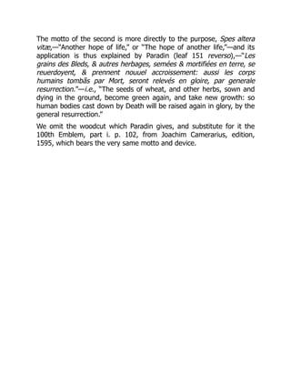

![to life, the wicked to judgment.”... “Elsewhere it is said, One Hope
survives, doubtless beyond the grave.”[107]
“Mort vivifiante,” of Messin, In Morte Vita, of Boissard, edition 1588,
pp. 38, 39, also receive their emblematical representation, from wheat
growing among the signs of death.
“En vain nous attendons la moisson, si le grain
Ne se pourrit au creux de la terre beschée.
Sans la corruption, la nature empeschée
Retient toute semence au ventre soubterrain.”
At present we must be content to say that the source of the motto
and device of the sixth knight has not been discovered. It remains for
us to conjecture, what is very far from being an improbability, that
Shakespeare had read Spenser’s Shepherd’s Calendar, published in
1579, and from the line, on page 364 of Moxon’s edition, for January
(l. 54),—
“Ah, God! that love should breed both ioy and paine!”—
and from the Emblem, as Spenser names it, Anchora speme,—“Hope
is my anchor,”—did invent for himself the sixth knight’s device, and its
motto, In hac spe vivo,—“In this hope I live.” The step from applying
so suitably the Emblems of other writers to the construction of new
ones would not be great; and from what he has actually done in the
invention of Emblems in the Merchant of Venice he would experience
very little trouble in contriving any Emblem that he needed for the
completion of his dramatic plans.
The Casket Scene and the Triumph Scene then justify our conclusion
that the correspondencies between Shakespeare and the Emblem
writers which preceded him are very direct and complete. It is to be
accepted as a fact that he was acquainted with their works, and
profited so much from them, as to be able, whenever the occasion
demanded, to invent and most fittingly illustrate devices of his own.](https://image.slidesharecdn.com/26607-250327174524-17abc328/85/Microsoft-Excel-365-Formulas-BarCharts-QuickStudy-1st-Edition-Curtis-Frye-19-320.jpg)


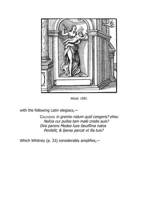
![“Medea loe with infante in her arme,
Whoe kil’de her babes, shee shoulde haue loued beste:
The swallowe yet, whoe did suspect no harme,
Hir Image likes, and hatch’d vppon her breste:[108]
And lifte her younge, vnto this tirauntes guide,
Whoe, peecemeale did her proper fruicte deuide.
Oh foolishe birde, think’ste thow, shee will haue care,
Vppon thy yonge? Whoe hathe her owne destroy’de,
And maie it bee, that shee thie birdes should spare?
Whoe slue her owne, in whome shee shoulde haue ioy’d.
Thow arte deceau’de, and arte a warninge good,
To put no truste, in them that hate theire blood.”
And to the same purport, from Alciat’s 193rd Emblem, are Whitney’s
lines (p. 29),—
“Medea nowe, and Progne, blusshe for shame:
By whome, are ment yow dames of cruell kinde
Whose infantes yonge, vnto your endlesse blame,
For mothers deare, do tyrauntes of yow finde:
Oh serpentes seede, each birde, and sauage brute,
Will those condempne, that tender not theire frute.”
The stanza of his 194th Emblem is adapted by Alciat, and by Whitney
after him (p. 163), to the motto,—
Pietas filiorum in parentes,—
“The reverence of sons towards their parents.”](https://image.slidesharecdn.com/26607-250327174524-17abc328/85/Microsoft-Excel-365-Formulas-BarCharts-QuickStudy-1st-Edition-Curtis-Frye-27-320.jpg)

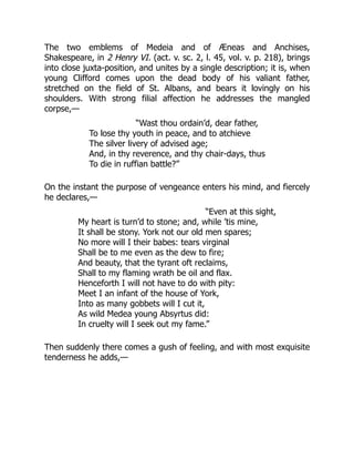
![Progne, or Procne, Medeia’s counterpart for cruelty, who placed the
flesh of her own son Itys before his father Tereus, is represented in
Aneau’s “Picta Poesis,” ed. 1552, p. 73, with a Latin stanza of ten lines,
and the motto, “Impotentis Vindictæ Foemina,”—The Woman of furious
Vengeance. In the Titus Andronicus (act. v. sc. 2, l. 192, vol. vi. p.
522) the fearful tale of Progne enters into the plot, and a similar
revenge is repeated. The two sons of the empress, Chiron and
Demetrius, who had committed atrocious crimes against Lavinia the
daughter of Titus, are bound, and preparations are made to inflict
such punishment as the world’s history had but once before heard of.
Titus declares he will bid their empress mother, “like to the earth
swallow her own increase.”
“This is the feast that I have bid her to,
And this the banquet she shall surfeit on;
For worse than Philomel you used my daughter,
And worse than Progne I will be revenged.”
’Tis a fearful scene, and the father calls,—
“And now prepare your throats. Lavinia, come,
[He cuts their throats.
Receive the blood: and when that they are dead,
Let me go grind their bones to powder small,
And with this hateful liquor temper it;
And in that paste let their vile heads be baked.
Come, come, be every one officious
To make this banquet; which I wish may prove
More stern and bloody than the Centaurs’ feast.”
A character from Virgil’s Æneid (bk. ii. lines 79–80; 195–8; 257–9),[109]
frequently introduced both by Whitney and Shakespeare, is that of the
traitor Sinon, who, with his false tears and lying words, obtained for
the wooden horse and its armed men admission through the walls and
within the city of Troy. Asia, he averred, would thus secure supremacy
over Greece, and Troy find a perfect deliverance. It is from the “Picta
Poesis” of Anulus (p. 18), that Whitney (p. 141) on one occasion](https://image.slidesharecdn.com/26607-250327174524-17abc328/85/Microsoft-Excel-365-Formulas-BarCharts-QuickStudy-1st-Edition-Curtis-Frye-31-320.jpg)

![“While throughe his foes, did boulde Brasidas thruste,
And thought with force, their courage to confounde:
Throughe targat faire, wherein he put his truste,
His manlie corpes receau’d a mortall wounde.
Beinge ask’d the cause, before he yeelded ghoste:
Quoth hee, my shielde, wherein I trusted moste.
Euen so it happes, wee ofte our bayne doe brue,
When ere wee trie, wee trust the gallante showe:
When frendes suppoas’d, do prooue them selues vntrue.
When Sinon false, in Damons shape dothe goe:
Then gulfes of griefe, doe swallowe vp our mirthe,
And thoughtes ofte times, doe shrow’d vs in the earthe.
* * * * * *
But, if thou doe inioye a faithfull frende,
See that with care, thou keepe him as thy life:
And if perhappes he doe, that may offende,
Yet waye thy frende: and shunne the cause of strife,
Remembringe still, there is no greater crosse;
Then of a frende, for, to sustaine the losse.
Yet, if this knotte of frendship be to knitte,
And Scipio yet, his Lelivs can not finde?
Content thy selfe, till some occasion fitte,
Allot thee one, according to thy minde:
Then trie, and truste: so maiste thou liue in rest,
But chieflie see, thou truste thy selfe the beste?”
And again, adopting the Emblem of John Sambucus, edition Antwerp,
1564, p. 184,[110]
and the motto,
Nusquam tuta fides,—
“Trustfulness is never sure,”](https://image.slidesharecdn.com/26607-250327174524-17abc328/85/Microsoft-Excel-365-Formulas-BarCharts-QuickStudy-1st-Edition-Curtis-Frye-34-320.jpg)


![Merces anguina,—“Reward from a serpent.”
“Frigore confectum quem rusticus inuenit anguem
Imprudens fotum recreat ecce sinu.
Immemor hic miserum lethale sauciat ictu:
Reddidit hìc vitam; reddidit ille necem.
Si benefacta locis malè, simplex mente, bonusq.:
Non benefacta quidem, sed malefacta puta.
Ingratis seruire nefas, gratisq. nocere:
Quod benè fit gratis, hoc solet esse lucro.”[111]
In several instances in his historical plays, Shakespeare very expressly
refers to this fable. On hearing that some of his nobles had made
peace with Bolingbroke, in Richard II. (act. iii. sc. 2, l. 129, vol. iv. p.
168), the king exclaims,—
“O villains, vipers, damn’d without redemption!
Dogs, easily won to fawn on any man!
Snakes, in my heart blood warm’d that sting my heart!”
In the same drama (act. v. sc. 3, l. 57, vol. iv. p. 210) York urges
Bolingbroke,—
“Forget to pity him, lest thy pity prove,
A serpent that will sting thee to the heart.”
And another, bearing the name of York, in 2 Henry VI. (act. iii. sc. 1, l.
343, vol. v. p. 162), declares to the nobles,—
“I fear me, you but warm the starved snake,
Who, cherish’d in your breasts, will sting your hearts.”
Also Hermia, Midsummer Night’s Dream (act. ii. sc. 2, l. 145, vol. ii. p.
225), when awakened from her trance-like sleep, calls on her beloved,
—](https://image.slidesharecdn.com/26607-250327174524-17abc328/85/Microsoft-Excel-365-Formulas-BarCharts-QuickStudy-1st-Edition-Curtis-Frye-37-320.jpg)
![“Help me, Lysander, help me! do thy best
To pluck this crawling serpent from my breast.”
Whitney combines Freitag’s and Reusner’s Emblems under one motto
(p. 189), In sinu alere serpentem,—“To nourish a serpent in the
bosom,”—but applies them to the siege of Antwerp in 1585 in a way
which Schiller’s famous history fully confirms:[112]
—“The government
of the citizens was shared among too many hands, and too strongly
influenced by a disorderly populace to allow any one to consider with
calmness, to decide with judgment, or to execute with firmness.”
The typical Sinon is here introduced by Whitney,—
“Thovghe, cittie stronge the cannons shotte dispise,
And deadlie foes, beseege the same in vaine:
Yet, in the walles if pining famine rise,
Or else some impe of Sinon, there remaine.
What can preuaile your bulwarkes? and your towers,
When, all your force, your inwarde foe deuoures.”
In fact, Sinon seems to have been the accepted representative of
treachery in every form; for when Camillus, at the siege of Faleria,
rewarded the Schoolmaster as he deserved for attempting to give up
his scholars into captivity, the occurence is thus described in the
Choice of Emblemes, p. 113,—
“With that, hee caus’de this Sinon to bee stripte,
And whippes, and roddes, vnto the schollers gaue:
Whome, backe againe, into the toune they whipte.”
Shakespeare is even more frequent in his allusions to this same Sinon.
The Rape of Lucrece, published in 1594, speaks of him as “the
perjured Sinon,” “the false Sinon,” “the subtle Sinon,” and avers (vol.
ix. p. 537, l. 1513),—](https://image.slidesharecdn.com/26607-250327174524-17abc328/85/Microsoft-Excel-365-Formulas-BarCharts-QuickStudy-1st-Edition-Curtis-Frye-38-320.jpg)