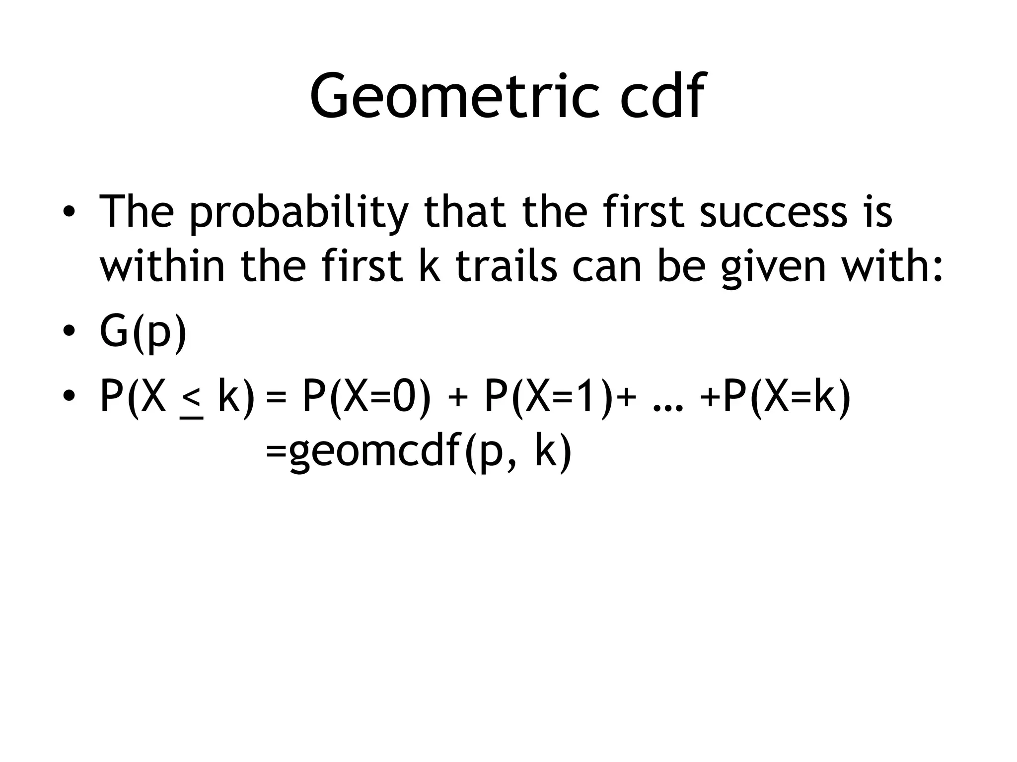
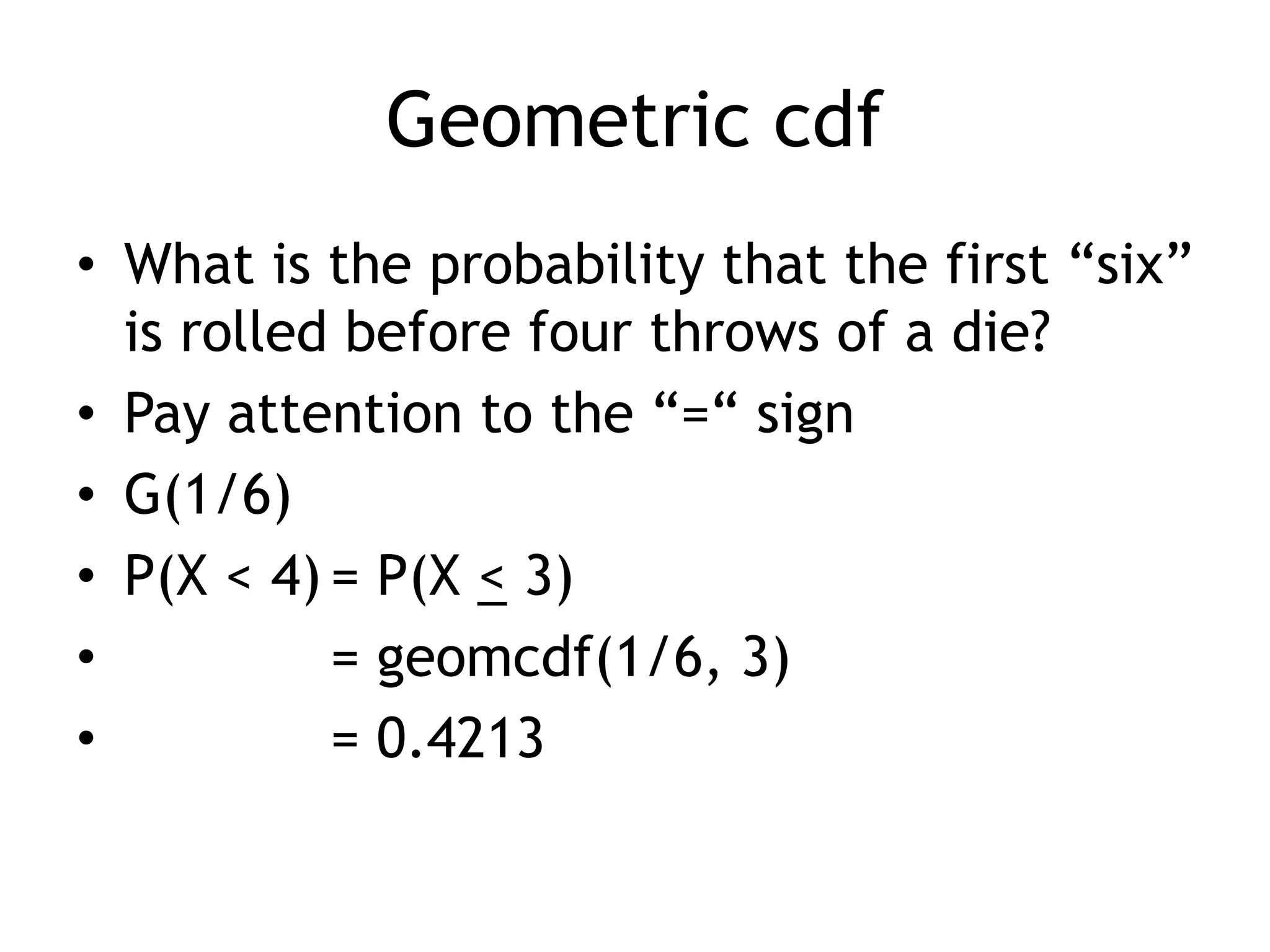
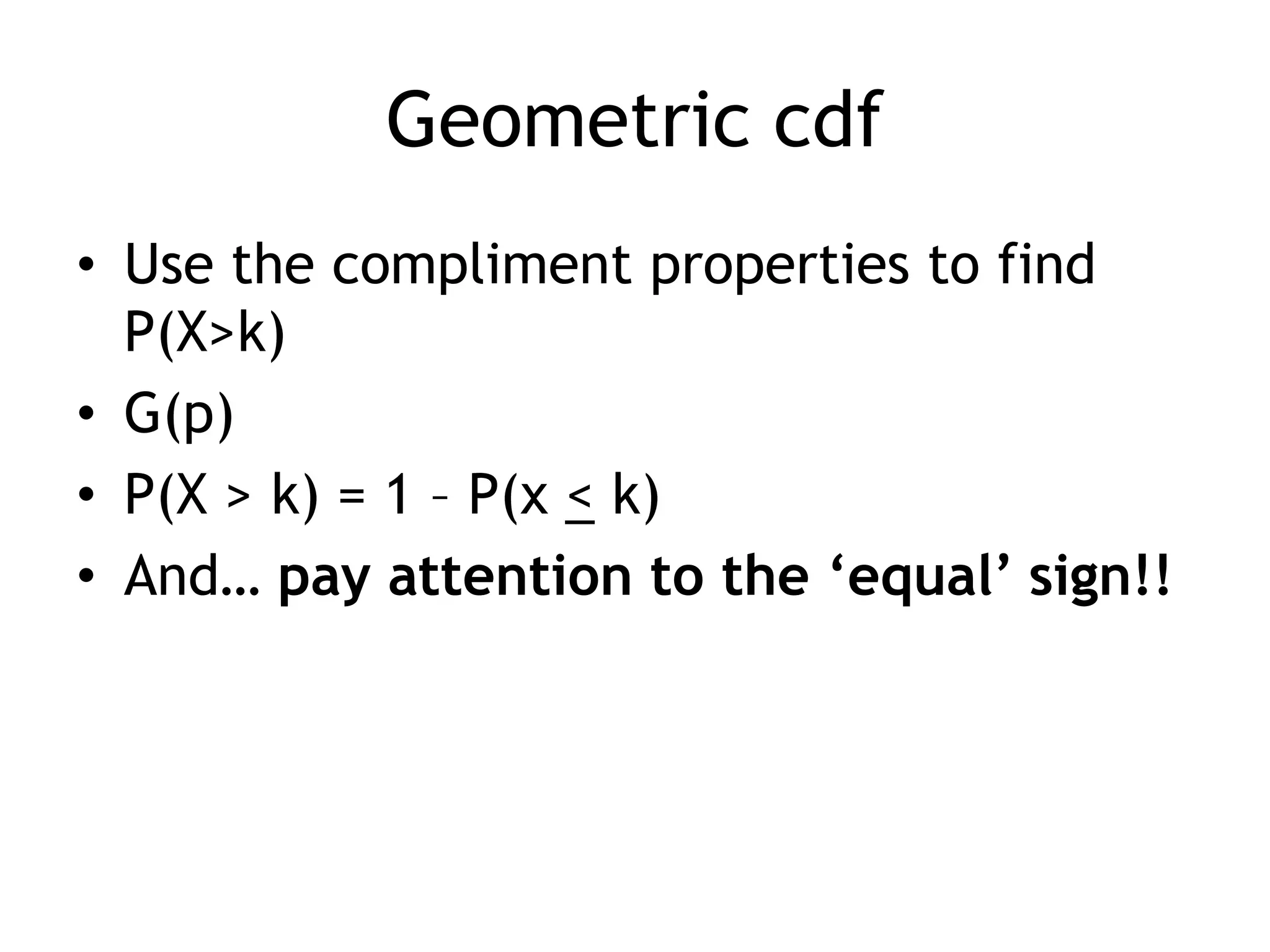
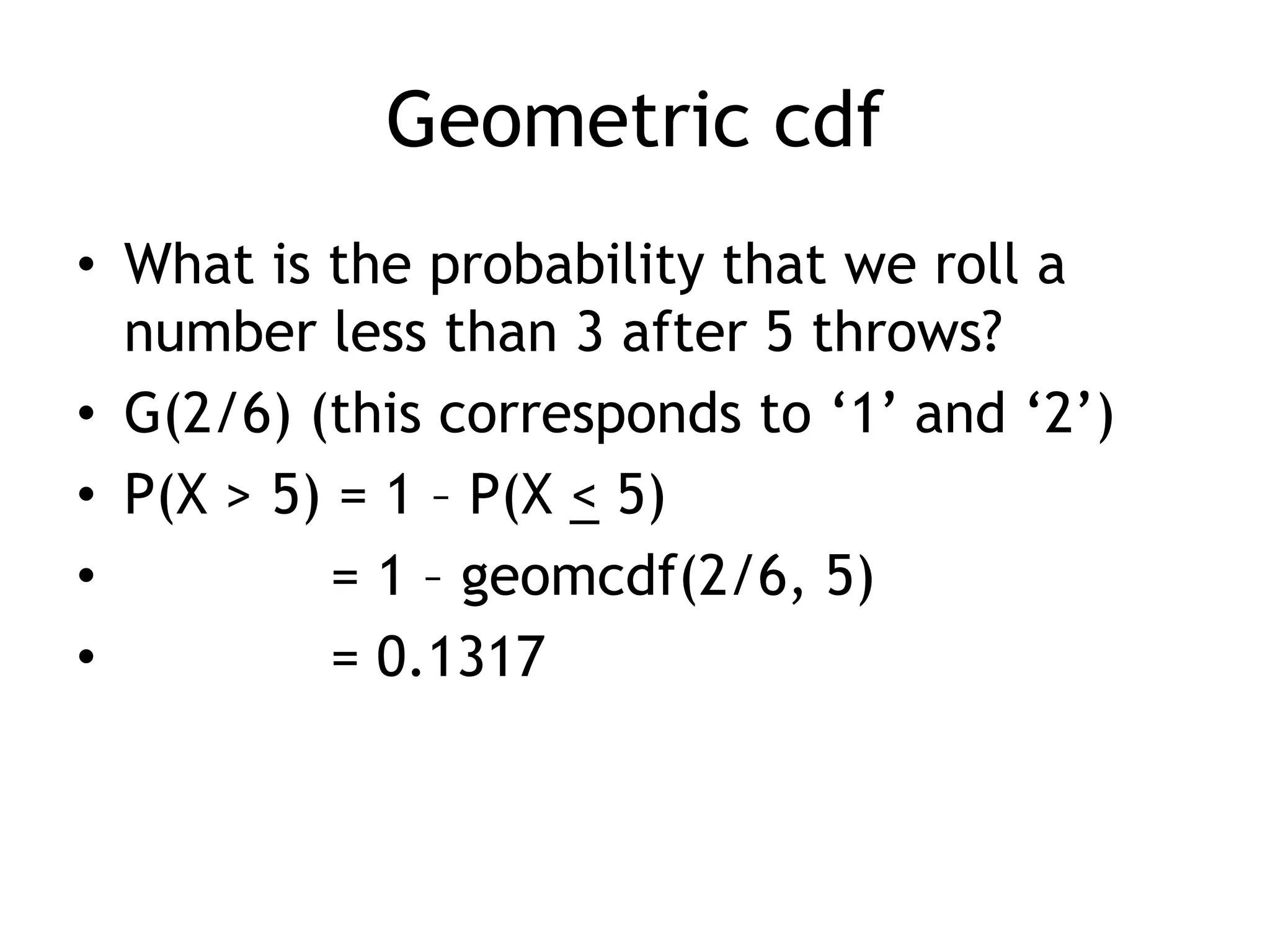
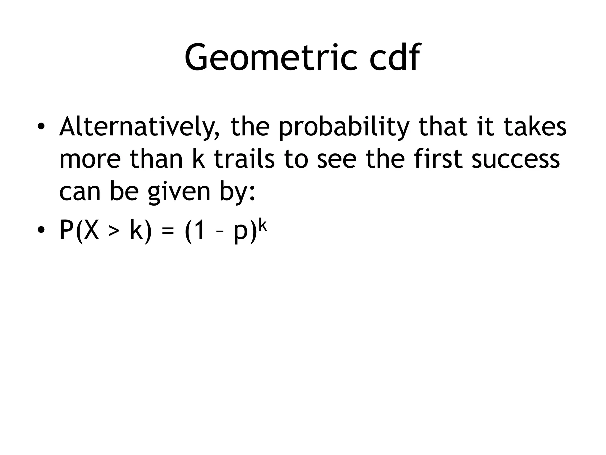
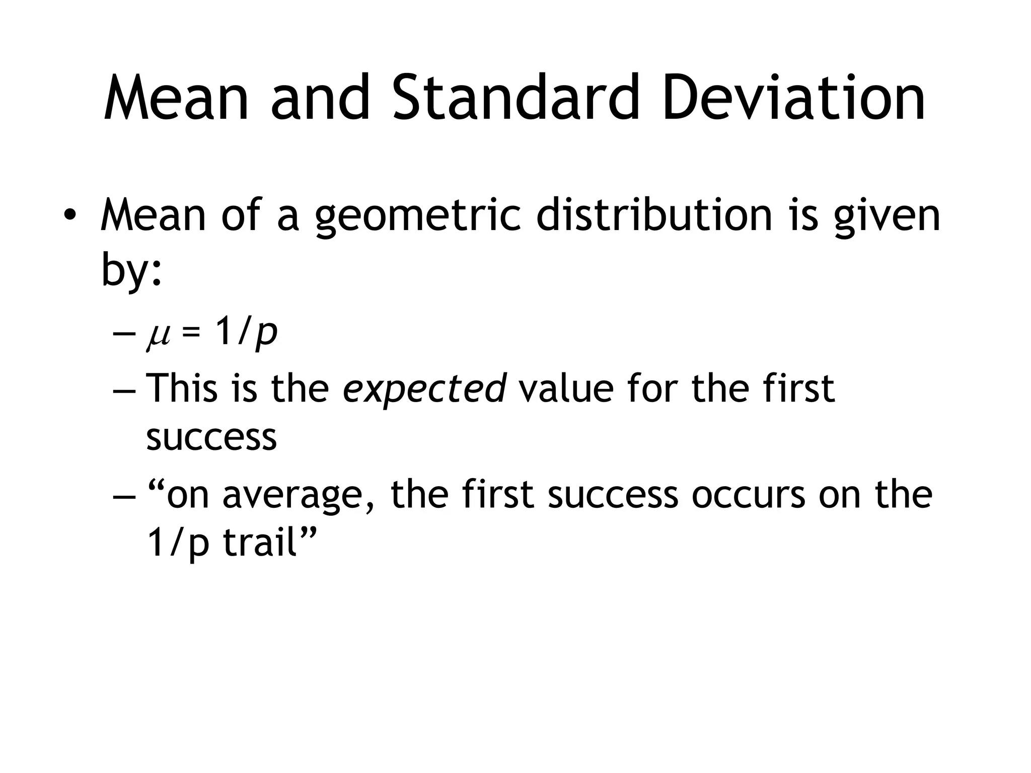
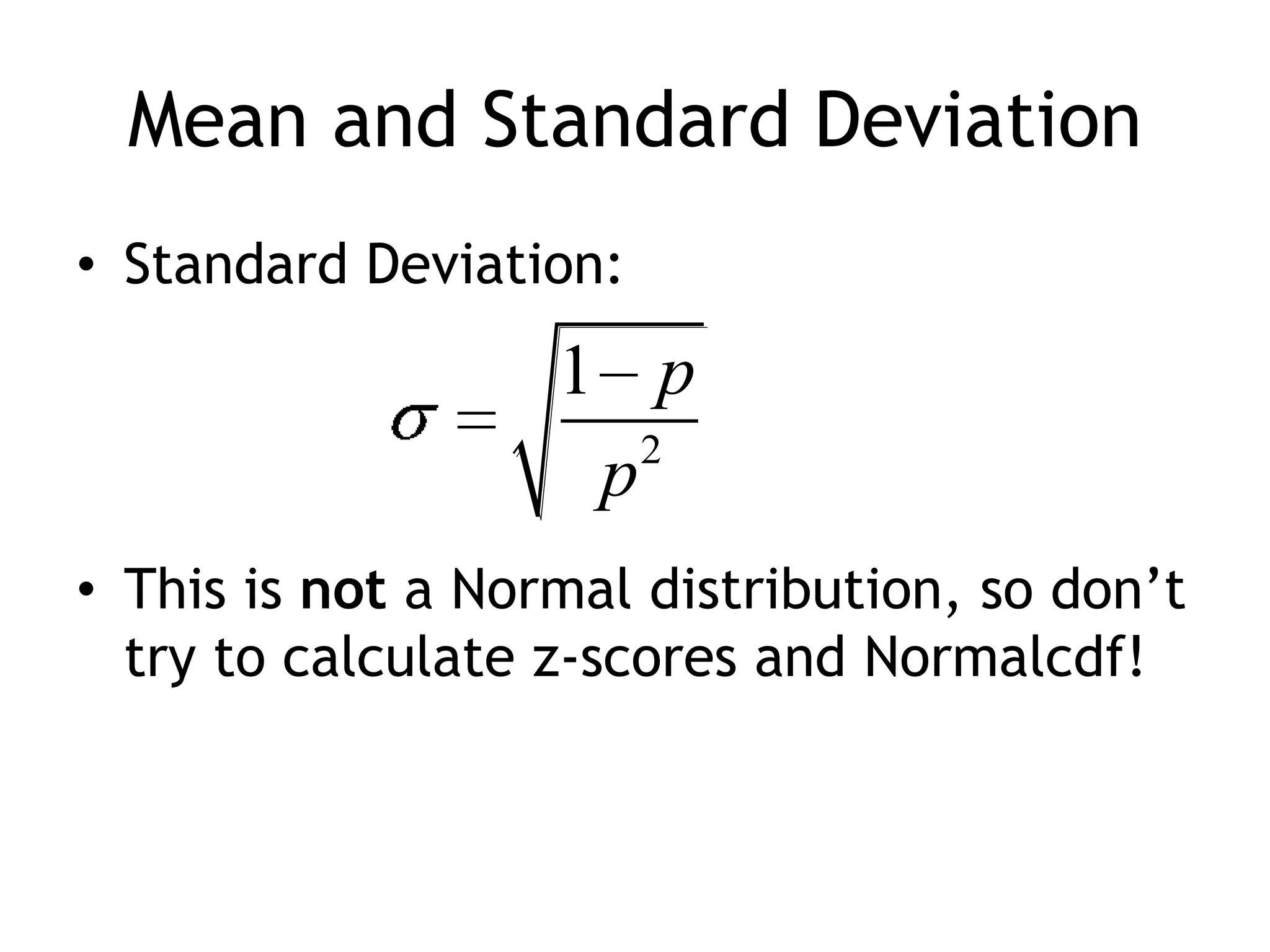
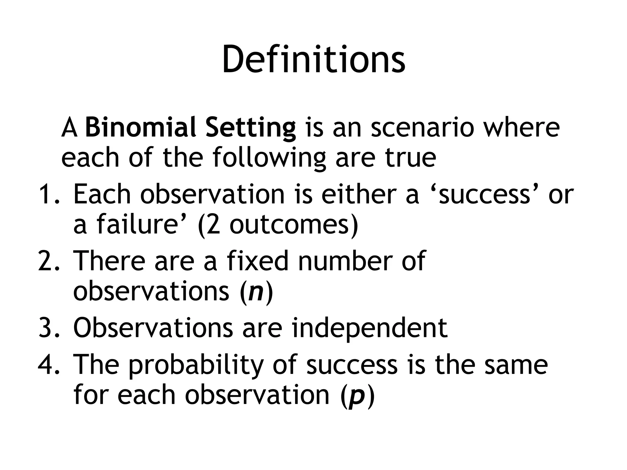
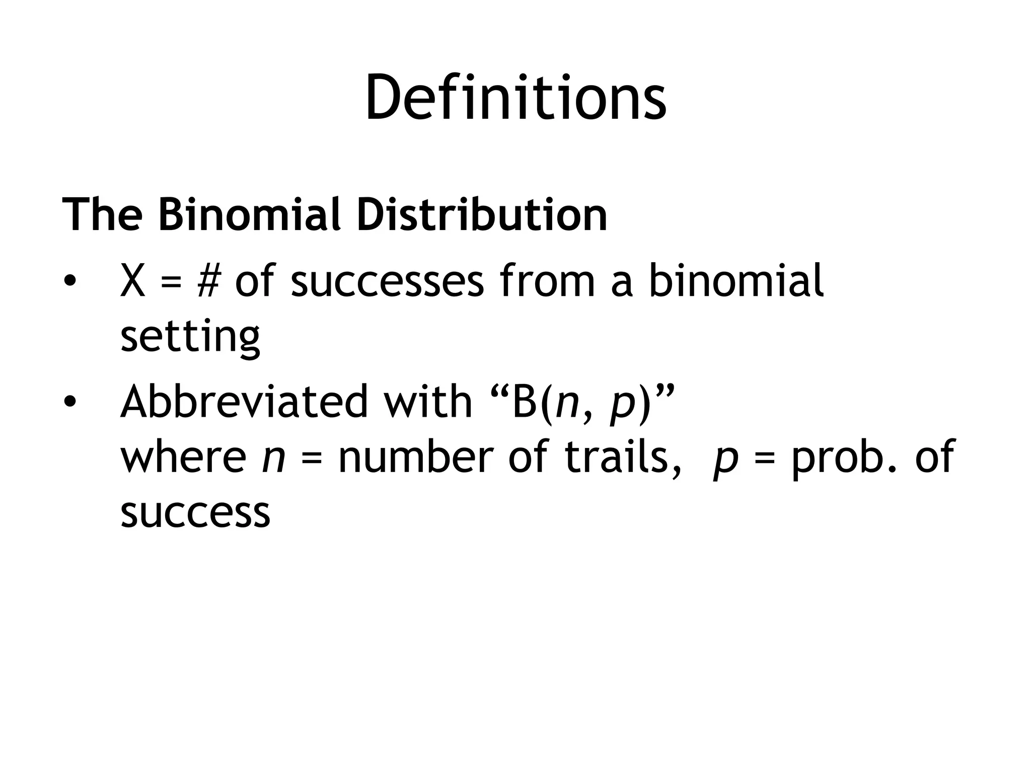
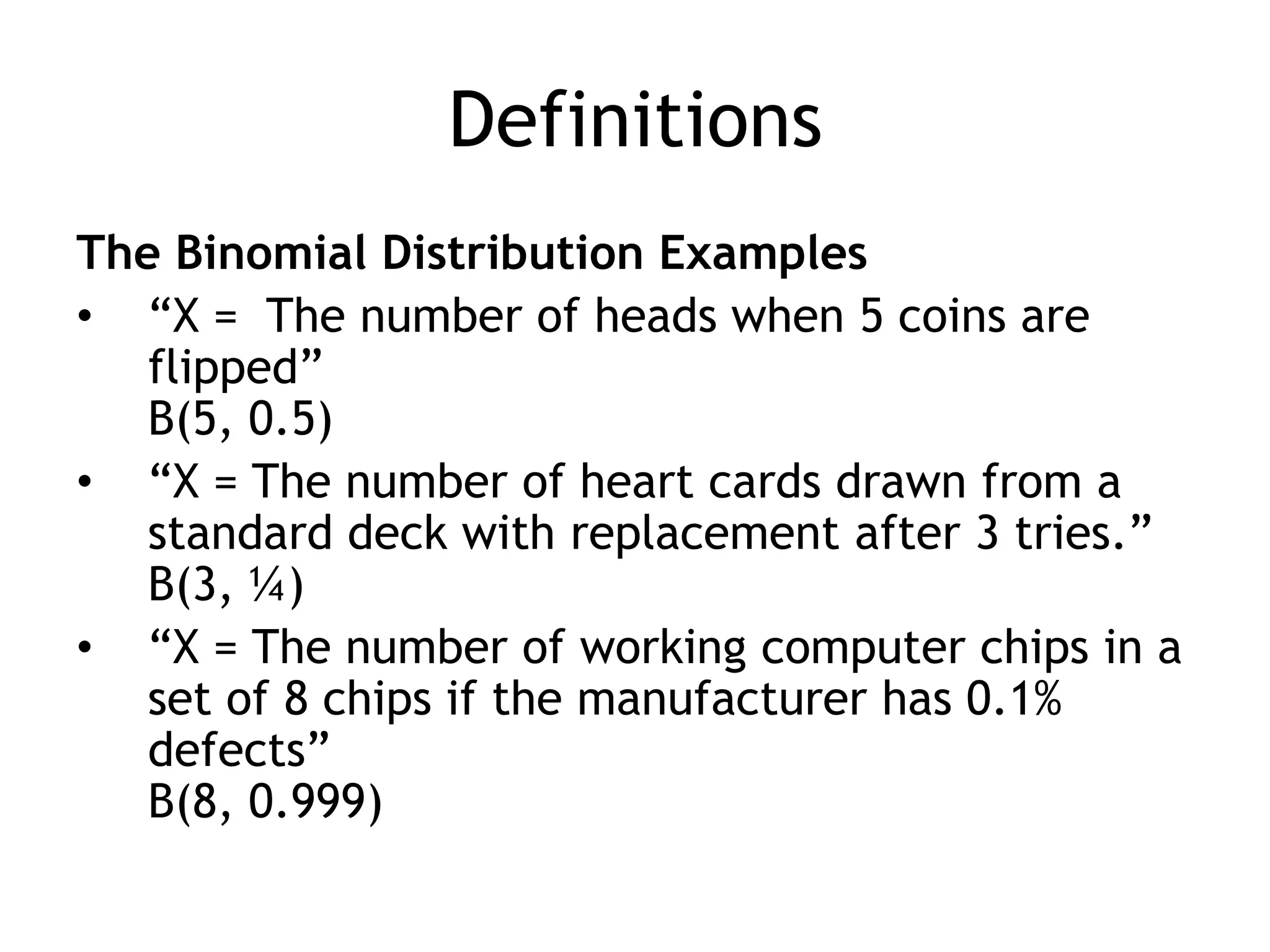
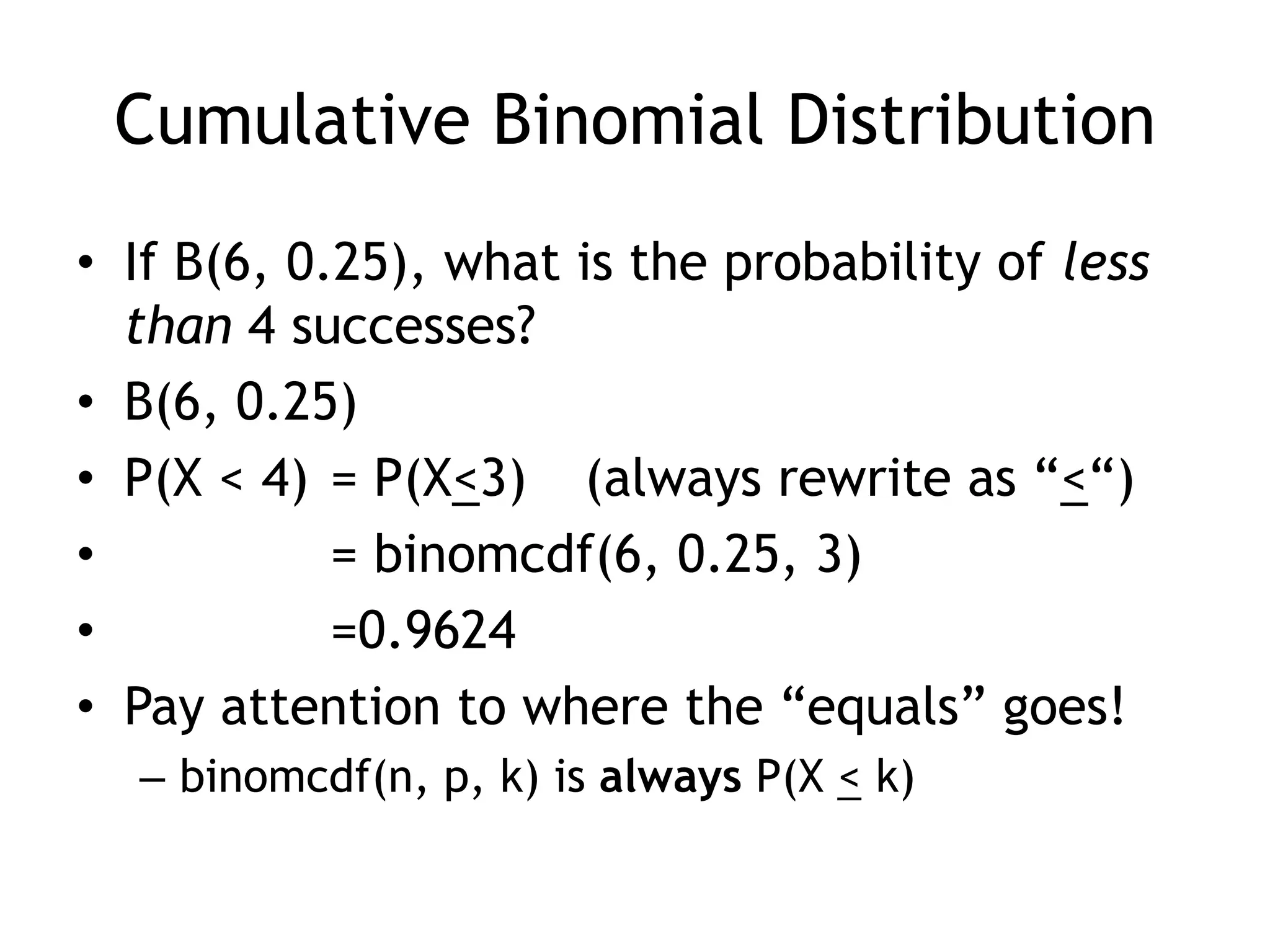
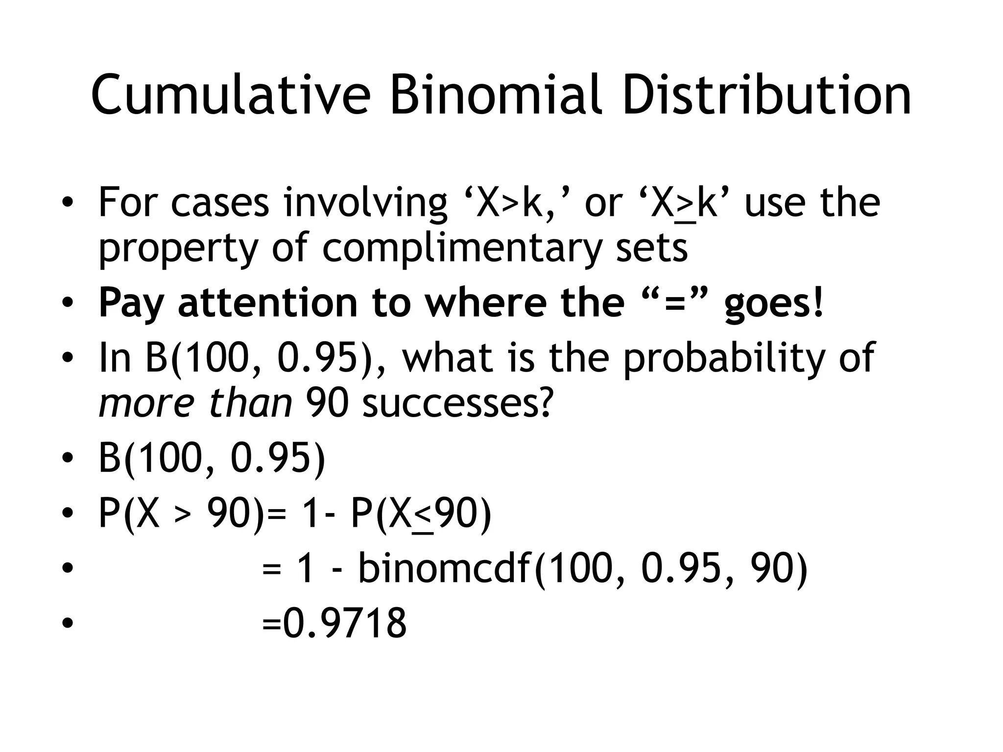
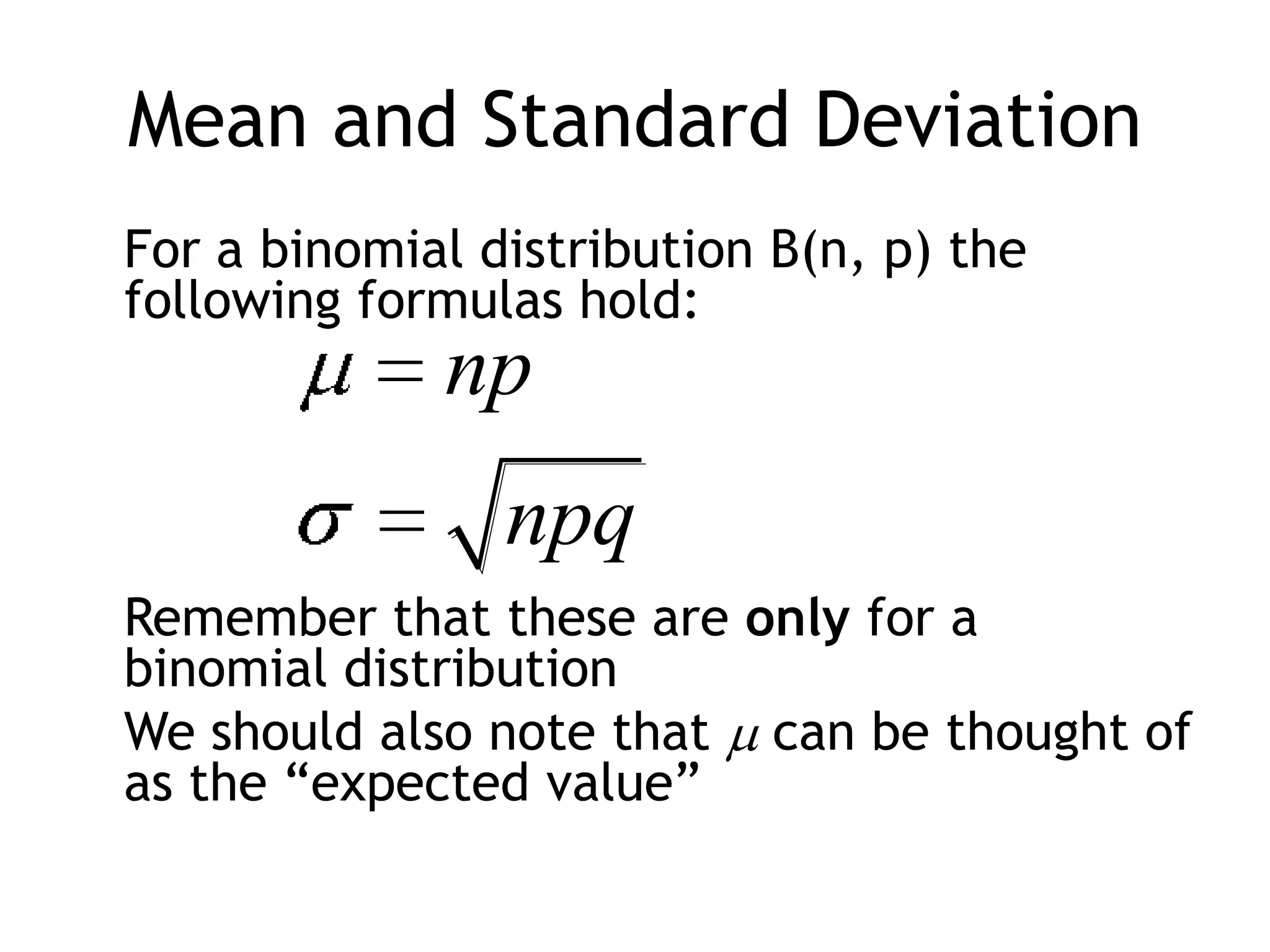
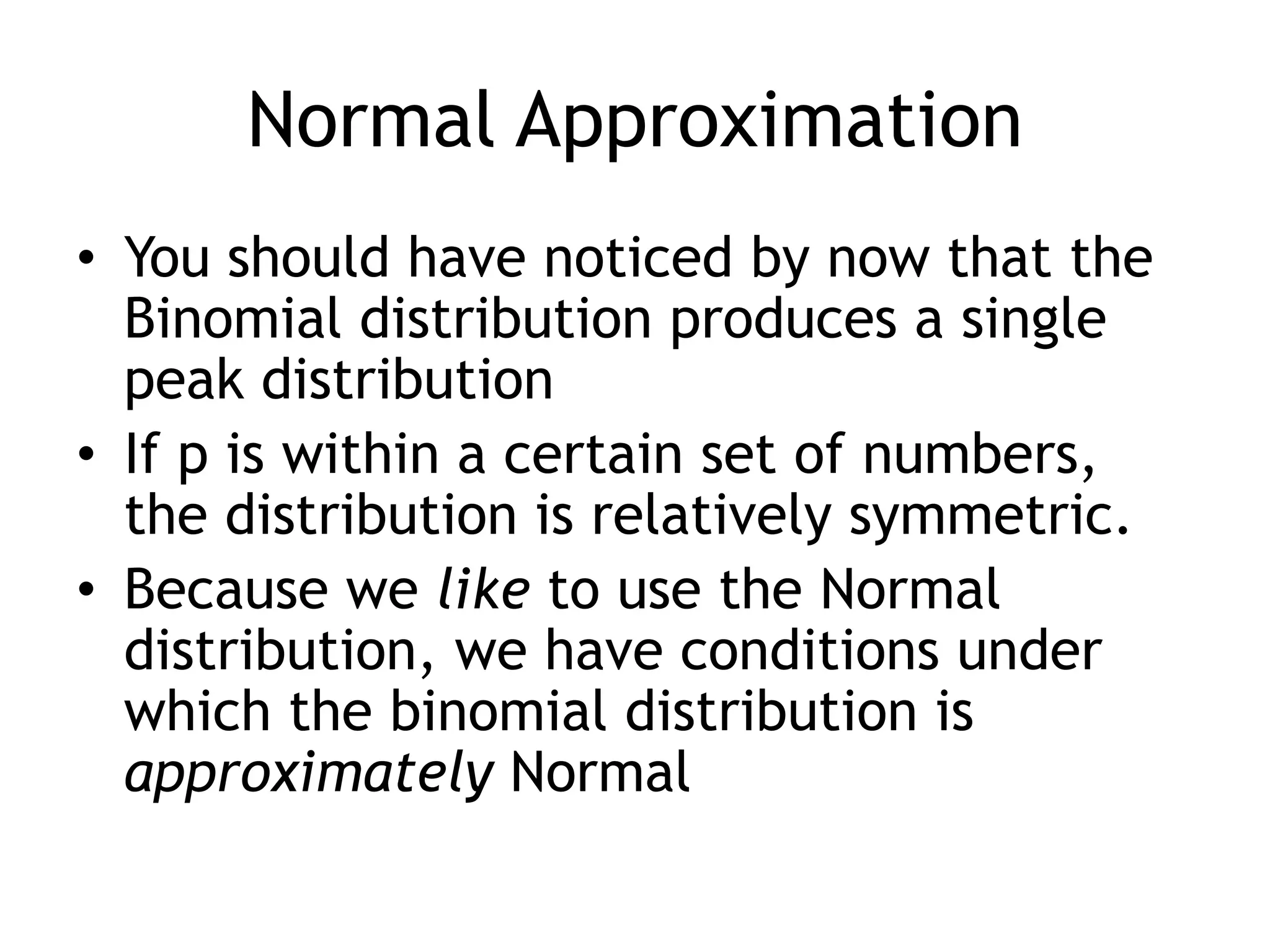
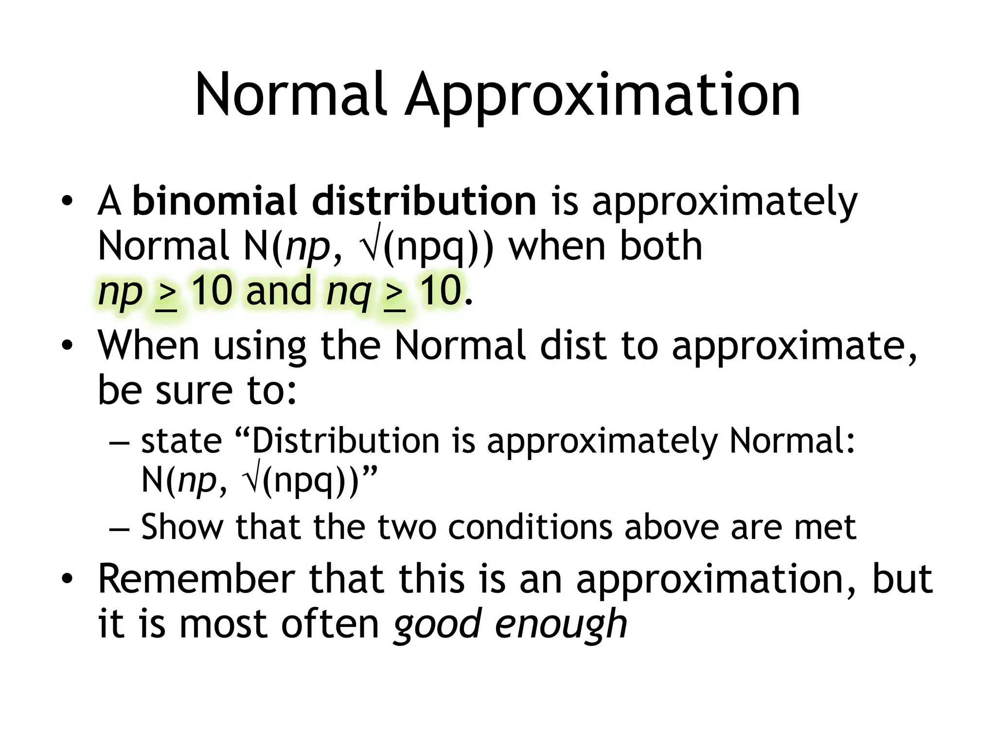
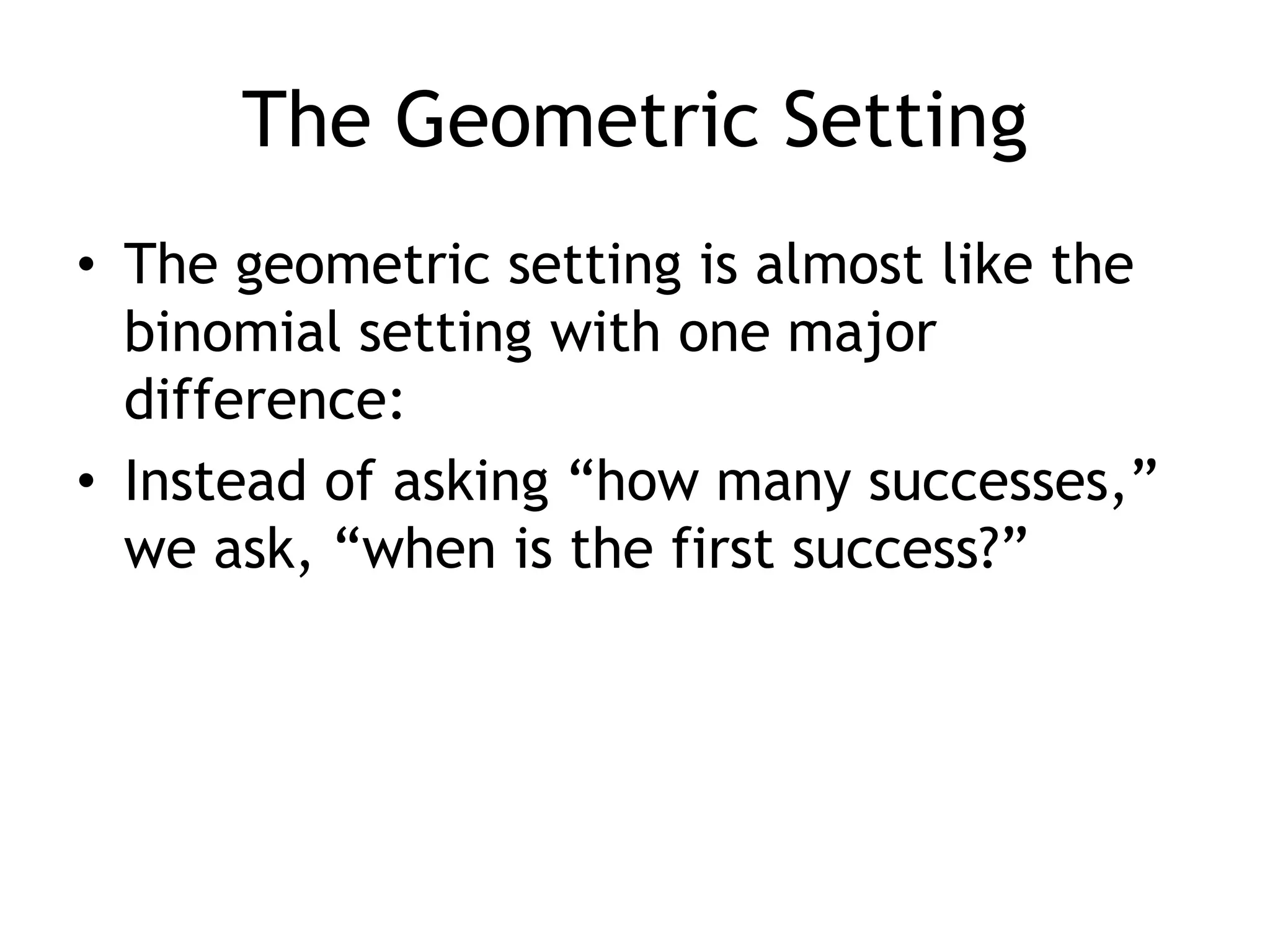
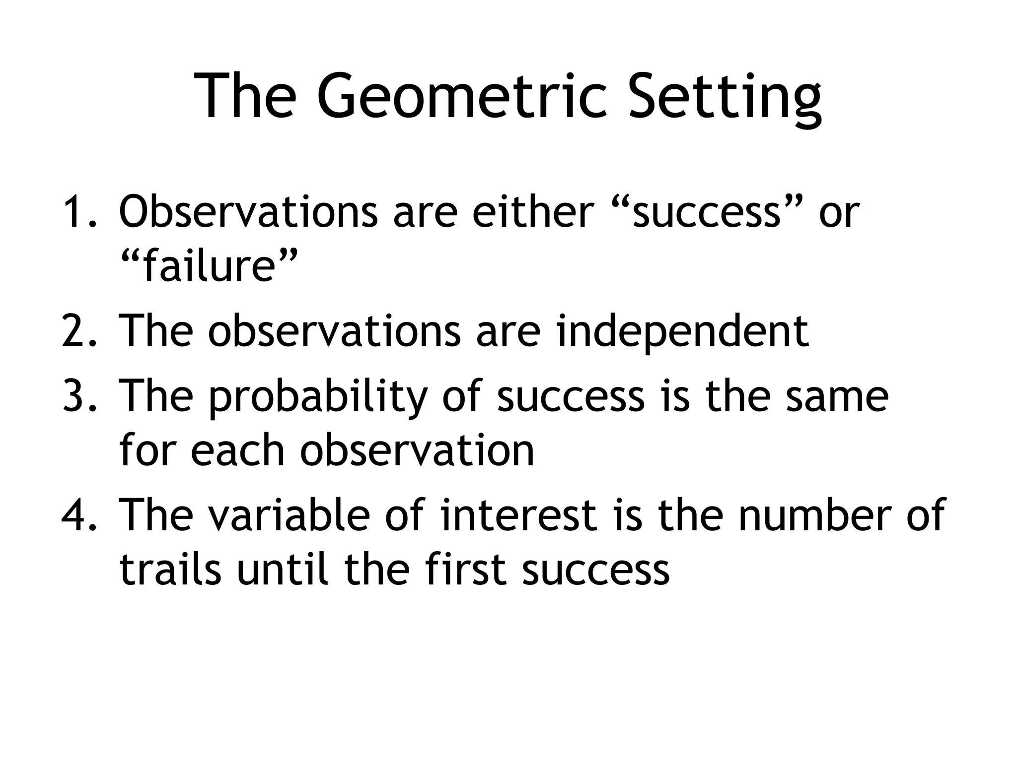
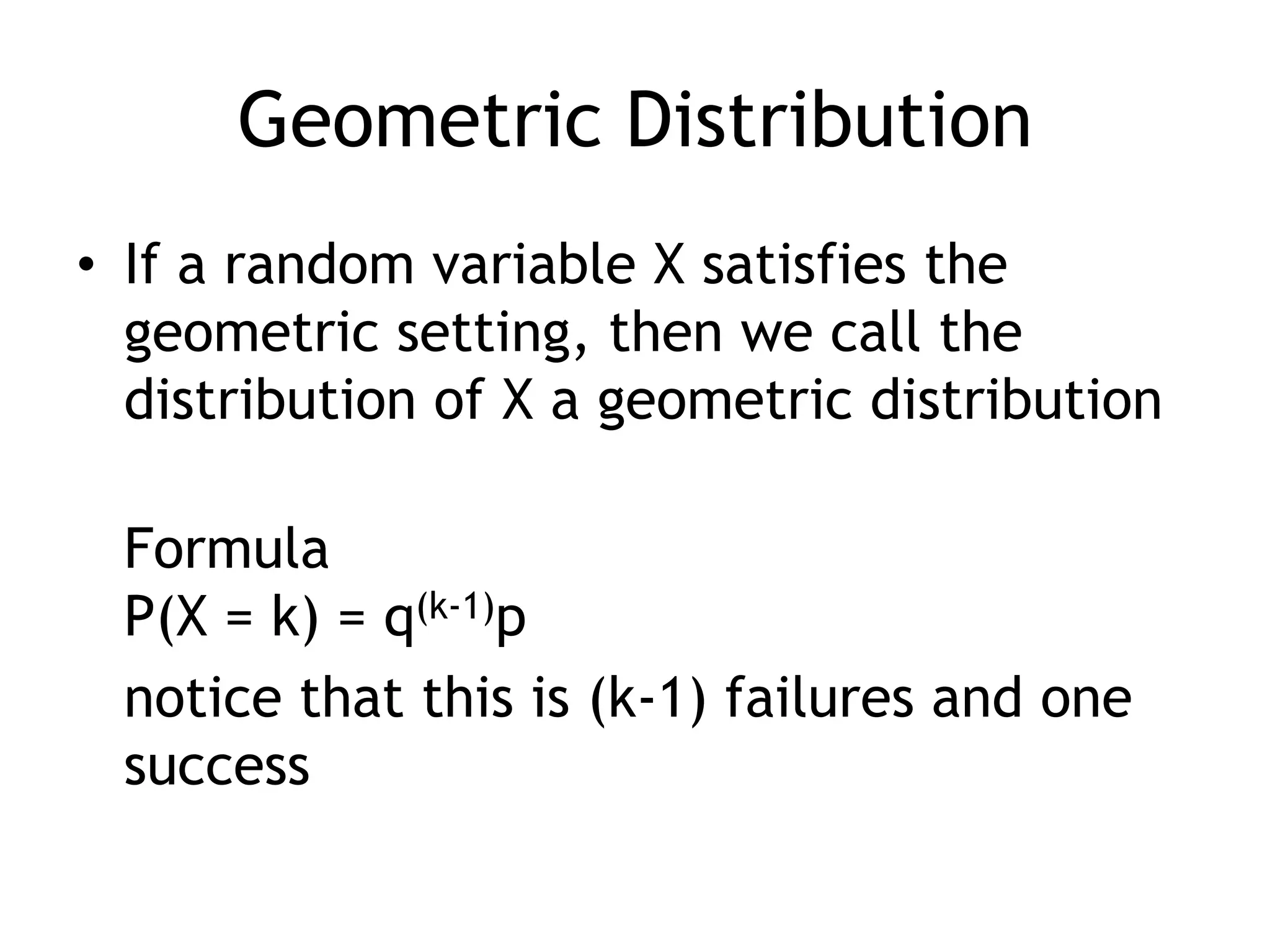
The document summarizes key concepts about the binomial and geometric distributions: The binomial distribution models the number of successes in a fixed number of yes/no trials where the probability of success is constant. The geometric distribution models the number of trials until the first success. Both have calculators functions and follow patterns for mean, standard deviation, and normal approximations. Formulas for probability mass and cumulative distribution functions are provided.

1. Chapter 8The Binomial and Geometric Distributions

2. 8.1 the Binomial Distribution

3. Definitions A Binomial Setting is an scenario where each of the following are trueEach observation is either a ‘success’ or a failure’ (2 outcomes)There are a fixed number of observations (n)Observations are independentThe probability of success is the same for each observation (p)

4. DefinitionsThe Binomial DistributionX = # of successes from a binomial settingAbbreviated with “B(n, p)”where n = number of trails, p = prob. of success

5. DefinitionsThe Binomial Distribution Examples“X = The number of heads when 5 coins are flipped”B(5, 0.5)“X = The number of heart cards drawn from a standard deck with replacement after 3 tries.”B(3, ¼)“X = The number of working computer chips in a set of 8 chips if the manufacturer has 0.1% defects”B(8, 0.999)

6. Sampling Distribution of a CountSuppose an SRS of size n is drawn from a population with a proportion p for success. Unless there is replacement, this isn’t binomial. Why? If the population is much greater than the sample size, then the sample has an approximate binomial distribution B(n, p)This helps use the binomial distribution in many cases that aren’t exactly a binomial setting.

7. Formulas for Binomial SettingsUsing a tree diagram, it is possible to formulate the binomial distribution.Example X = number of heads when a loaded coin is flipped 3 times (P(heads = 0.3)

8. Formulas for Binomial SettingsSetting is B(3, .3)Sample Space-HHH, HHT, HTH, THH, HTT, THT, TTH, TTTProbabilitiesP(X = 3) = 0.027, P(X = 2) = 3·(.3)2(.7) = 0.189, P(X = 1) = 3·(.3)(.7)2=0.441, P(X = 0) = (.7)3=0.343Unfortunately, this works best only for simple settings

9. Formulas for Binomial SettingsBinomial coefficientThis is a part of the formula for the binomial distribution.n = # trails, k = # of successYou may have seen this formula before!

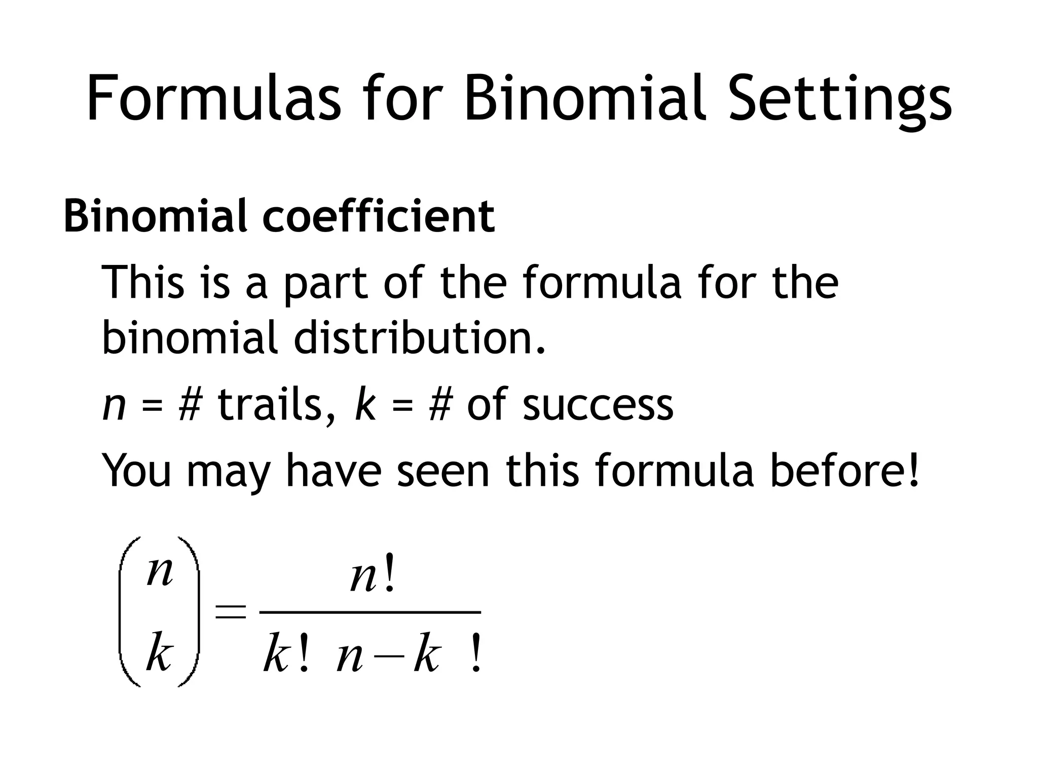
10. Formulas for Binomial SettingsBinomial coefficientYour calculator can find this coefficient for you[math] , “PRB,” “nCr” example

11. Formulas for Binomial SettingsBinomial ProbabilityIf we have a binomial setting B(n, p) and we want to know P(X = k)

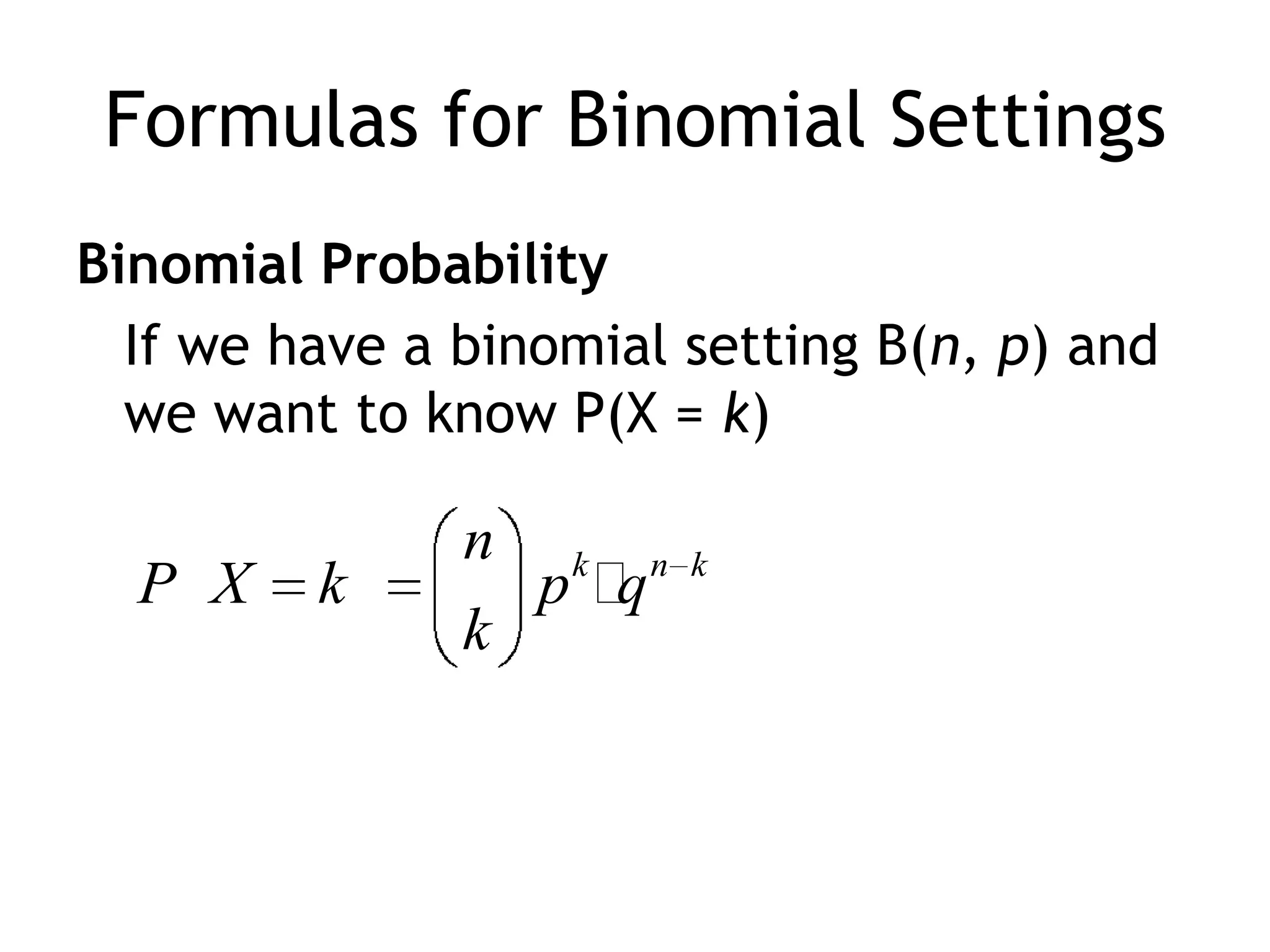
12. Formulas for Binomial SettingsBinomial ProbabilityActually your calculator is very efficient in these caculations.The binomial magic is [2nd] [vars] (dist), “binompdf(“ Again assuming B(n. p)

13. Some Alphabet Soup“pdf” means “probability distribution function,” which is exactly what we are doing!“binompdf” is the “binomial probability function”This is a discrete probability distribution“cdf” means “cumulative distribution function”This will add together a number of successes.

14. Cumulative Binomial DistributionFor the question, “if B(n, p), what is the probability k or less successes?”B(5, 0.33) P(X < 2) = P(X=0) + P(X=1) + P(X=2) = binomcdf(5, 0.33, 2)Pay attention to where the “equals” goes!Binomcdf(n,p, k) is always P(X < k)

15. Cumulative Binomial DistributionIf B(6, 0.25), what is the probability of less than 4 successes?B(6, 0.25)P(X < 4) = P(X<3) (always rewrite as “<“) = binomcdf(6, 0.25, 3) =0.9624Pay attention to where the “equals” goes!binomcdf(n, p, k) is always P(X < k)

16. Cumulative Binomial DistributionFor cases involving ‘X>k,’ or ‘X>k’ use the property of complimentary setsPay attention to where the “=” goes!In B(100, 0.95), what is the probability of more than 90 successes?B(100, 0.95)P(X > 90)= 1- P(X<90) = 1 - binomcdf(100, 0.95, 90) =0.9718

17. Mean and Standard Deviation For a binomial distribution B(n, p) the following formulas hold:Remember that these are only for a binomial distribution We should also note that  can be thought of as the “expected value”

18. Normal ApproximationYou should have noticed by now that the Binomial distribution produces a single peak distributionIf p is within a certain set of numbers, the distribution is relatively symmetric.Because we like to use the Normal distribution, we have conditions under which the binomial distribution is approximately Normal

19. Normal ApproximationA binomial distribution is approximately Normal N(np, (npq)) when both np>10 and nq> 10.When using the Normal dist to approximate, be sure to: state “Distribution is approximately Normal: N(np, (npq))”Show that the two conditions above are metRemember that this is an approximation, but it is most often good enough

20. 8.2 The Geometric Distribution

21. The Geometric SettingThe geometric setting is almost like the binomial setting with one major difference:Instead of asking “how many successes,” we ask, “when is the first success?”

22. The Geometric SettingObservations are either “success” or “failure”The observations are independentThe probability of success is the same for each observationThe variable of interest is the number of trails until the first success

23. Geometric DistributionIf a random variable X satisfies the geometric setting, then we call the distribution of X a geometric distribution FormulaP(X = k) = q(k-1)pnotice that this is (k-1) failures and one success

24. Geometric Distribution on the TILike the Binomial Distribution, the Geometric Distribution is found at[2nd] [var] (dist)for G(p)P(X=k) = q(k-1)p = geompdf(p,k)

25. Geometric cdfThe probability that the first success is within the first k trails can be given with:G(p)P(X < k) = P(X=0) + P(X=1)+ … +P(X=k) =geomcdf(p, k)

26. Geometric cdfWhat is the probability that the first “six” is rolled before four throws of a die?Pay attention to the “=“ signG(1/6)P(X < 4) = P(X < 3) = geomcdf(1/6, 3) = 0.4213

27. Geometric cdfUse the compliment properties to find P(X>k)G(p)P(X > k) = 1 – P(x < k)And… pay attention to the ‘equal’ sign!!

28. Geometric cdfWhat is the probability that we roll a number less than 3 after 5 throws?G(2/6) (this corresponds to ‘1’ and ‘2’)P(X > 5) = 1 – P(X < 5) = 1 – geomcdf(2/6, 5) = 0.1317

29. Geometric cdfAlternatively, the probability that it takes more than k trails to see the first success can be given by:P(X > k) = (1 – p)k

30. Mean and Standard DeviationMean of a geometric distribution is given by: = 1/pThis is the expected value for the first success“on average, the first success occurs on the 1/p trail”

31. Mean and Standard DeviationStandard Deviation:This is not a Normal distribution, so don’t try to calculate z-scores and Normalcdf!