The document describes multiple regression models and their applications. It begins by defining a general multiple regression model that relates a dependent variable to multiple predictor variables. It then discusses key aspects of multiple regression models like regression coefficients, the regression function, polynomial regression models, and qualitative predictor variables. The document provides examples of applying multiple regression to model lung capacity based on variables like height, age, gender, and activity level. It describes building different regression models and evaluating their fit and significance.

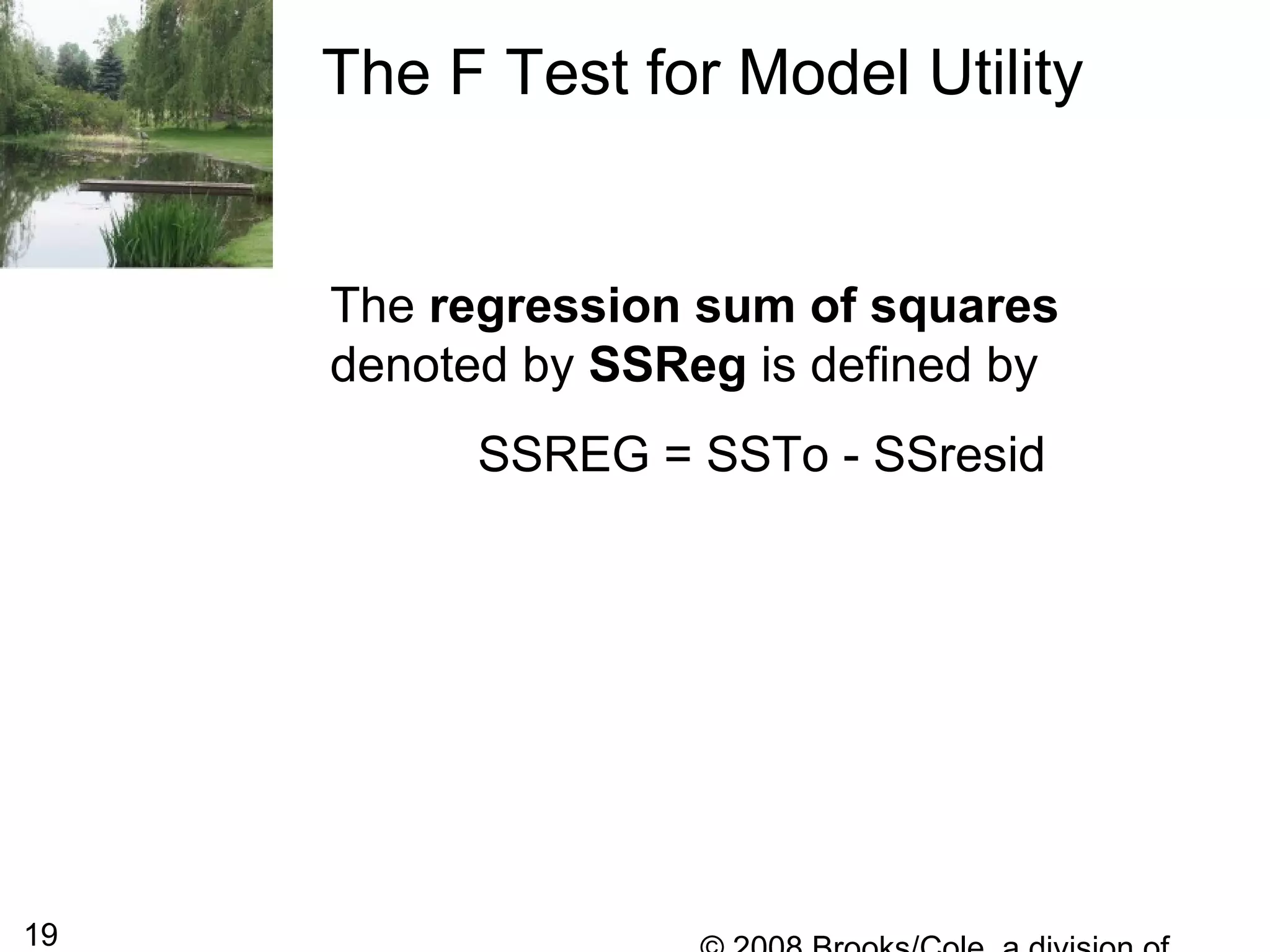
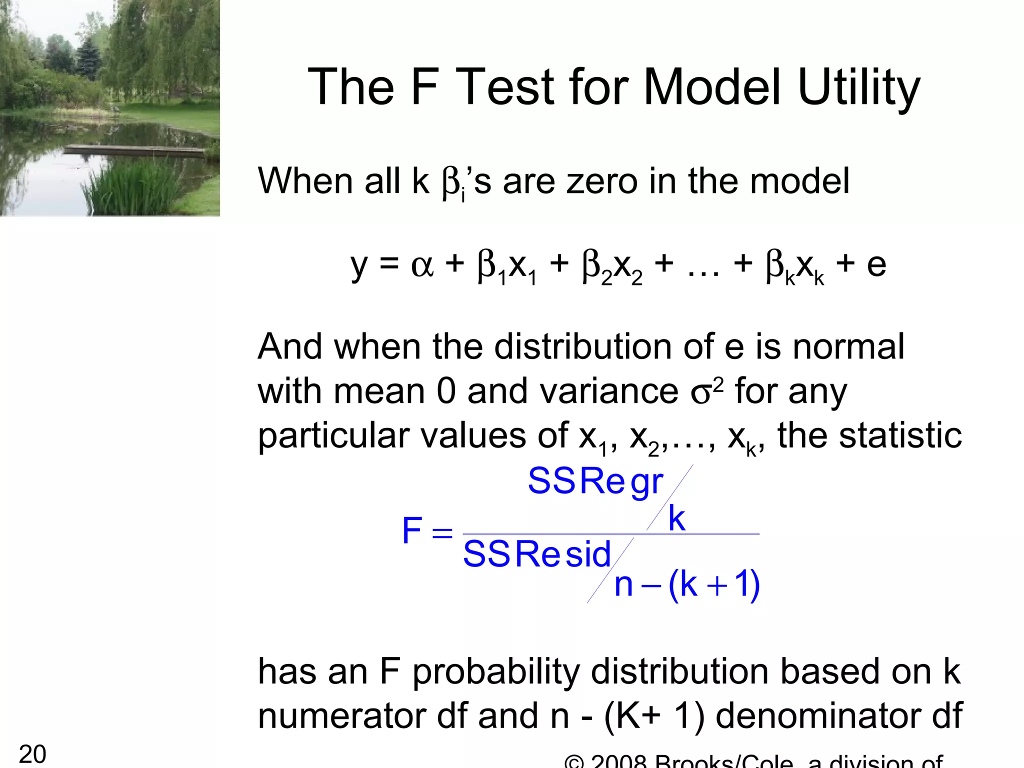
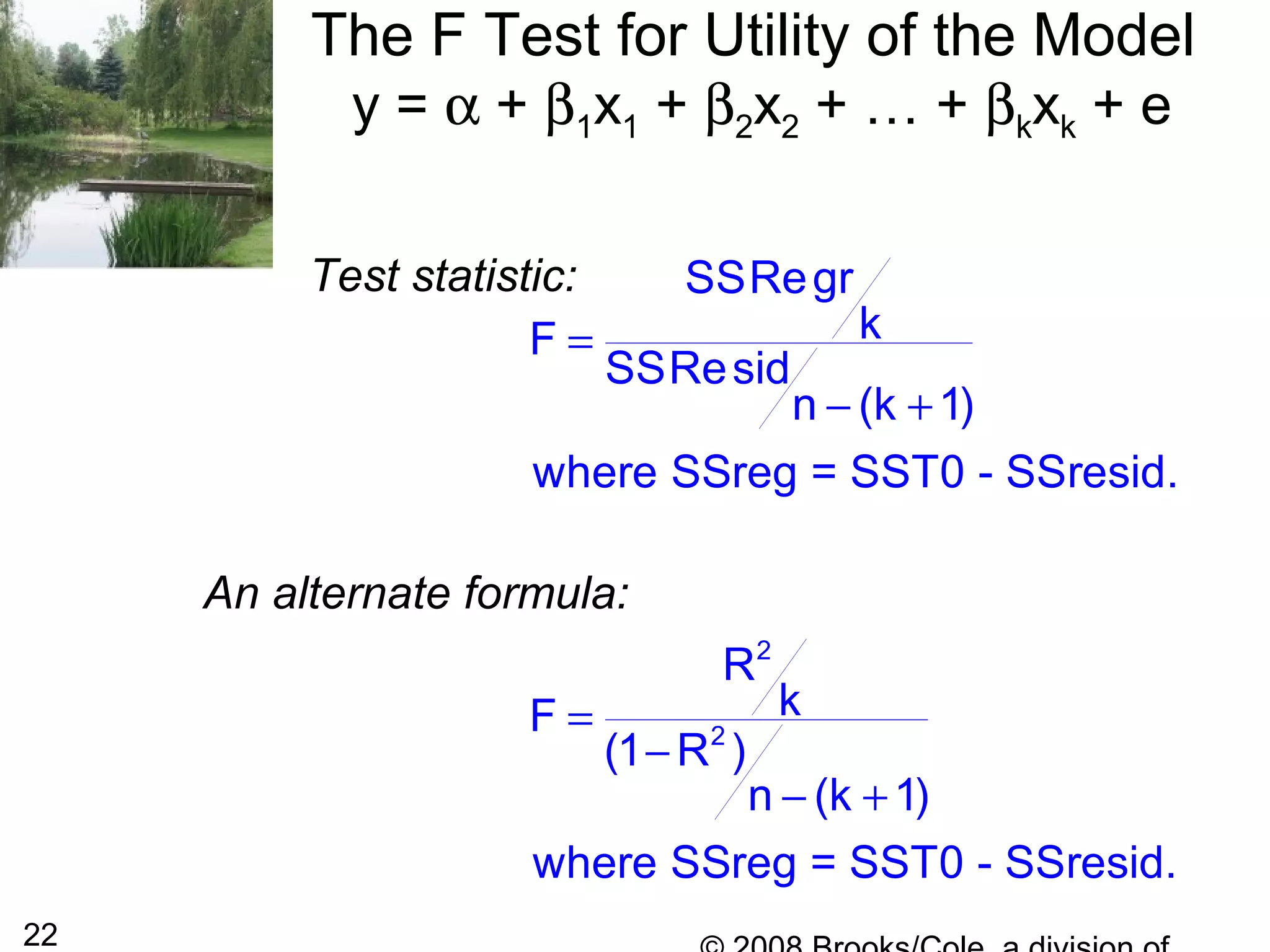
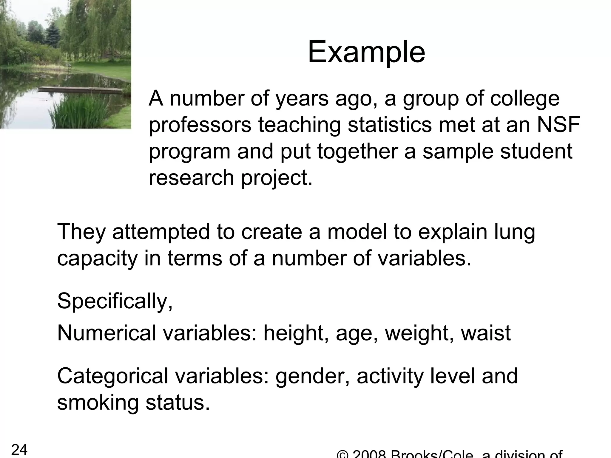
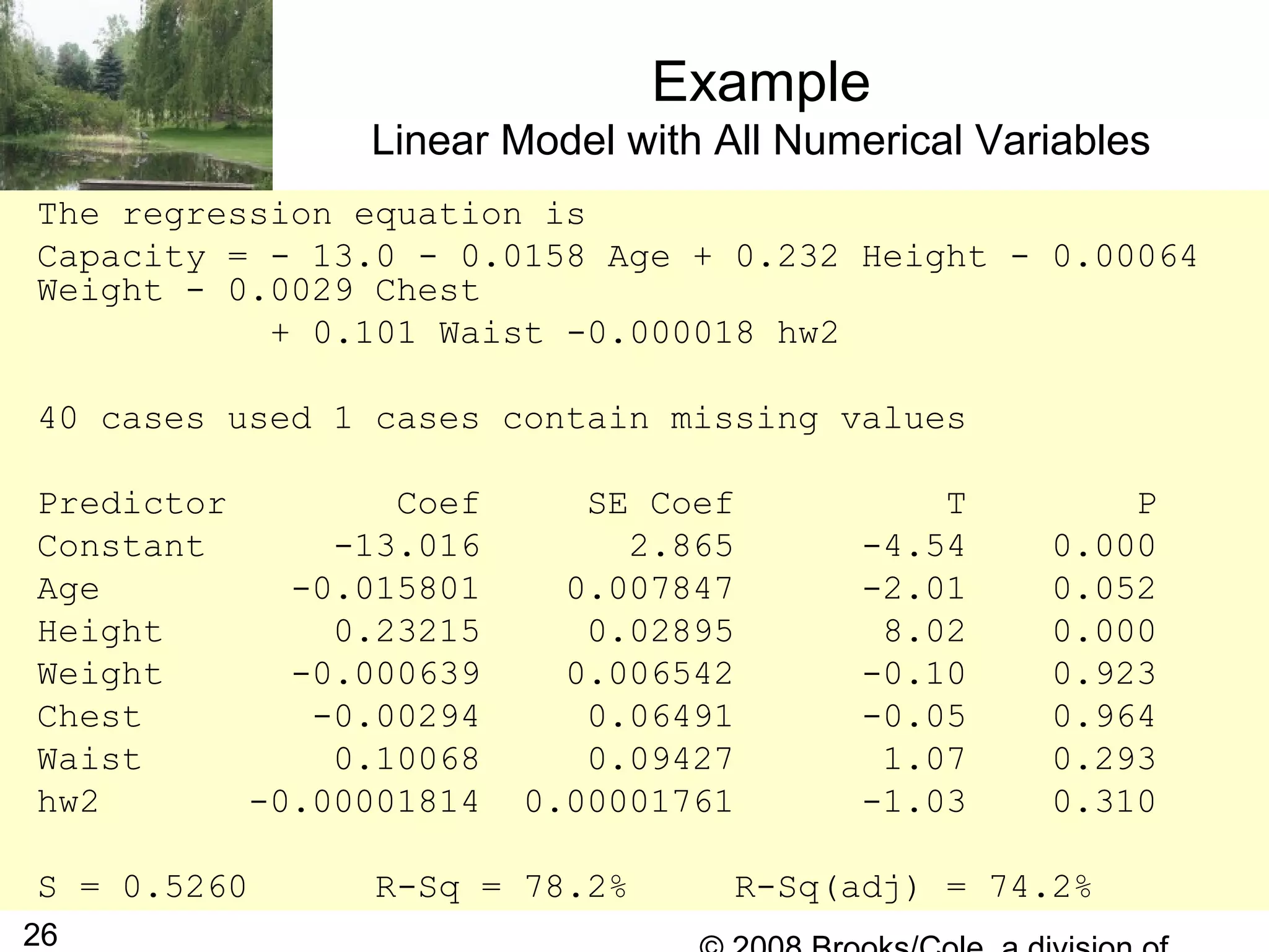
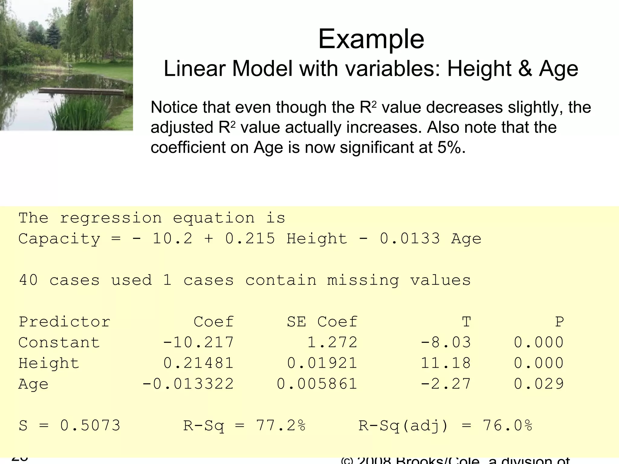
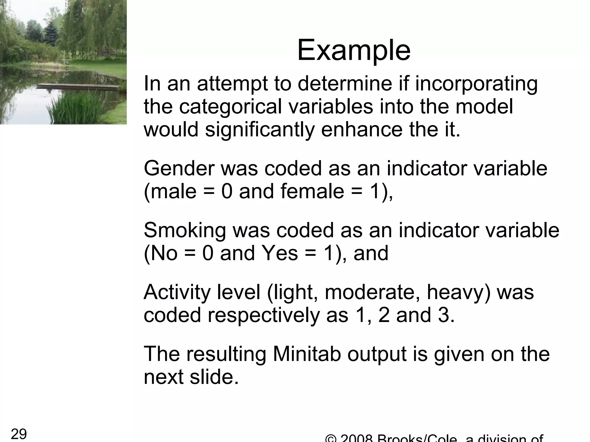
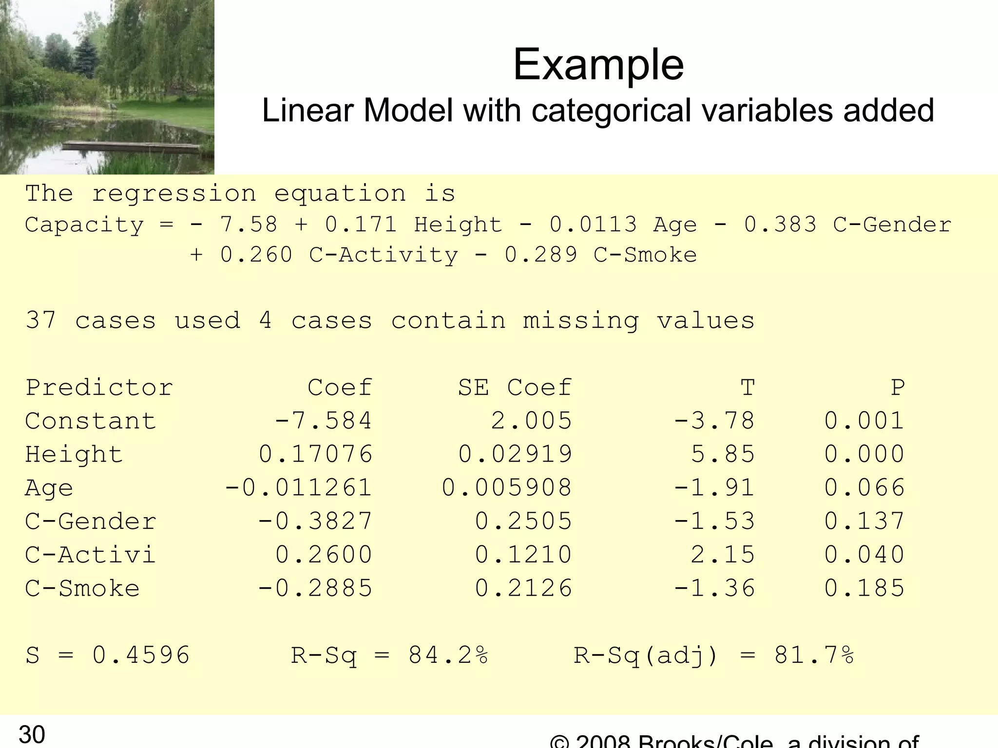
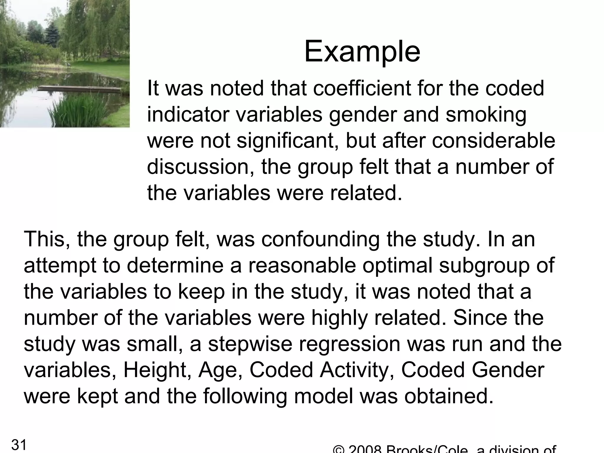
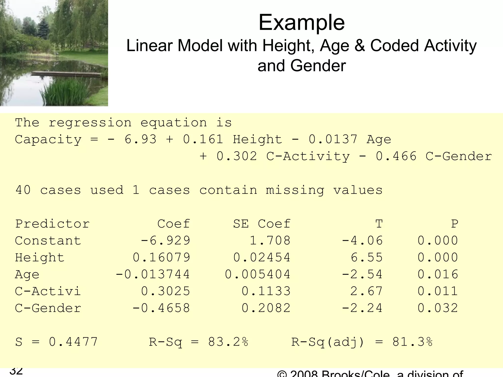
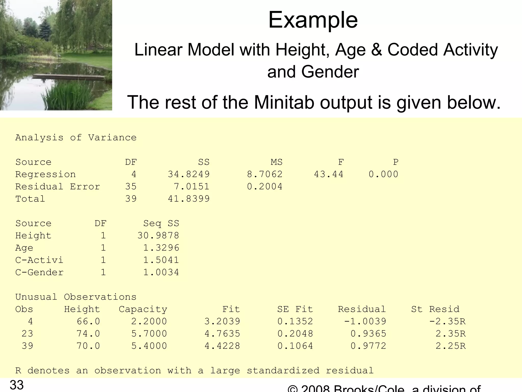
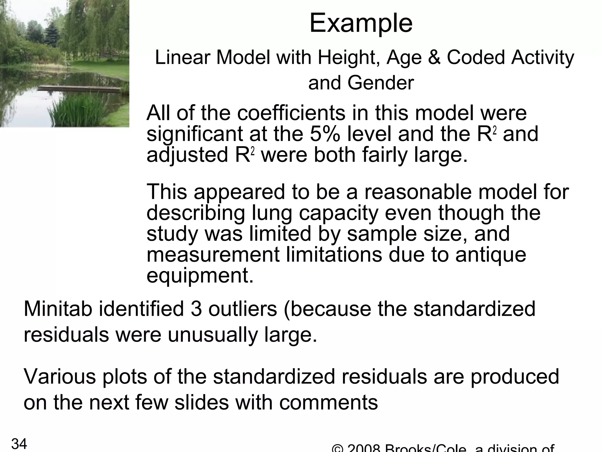
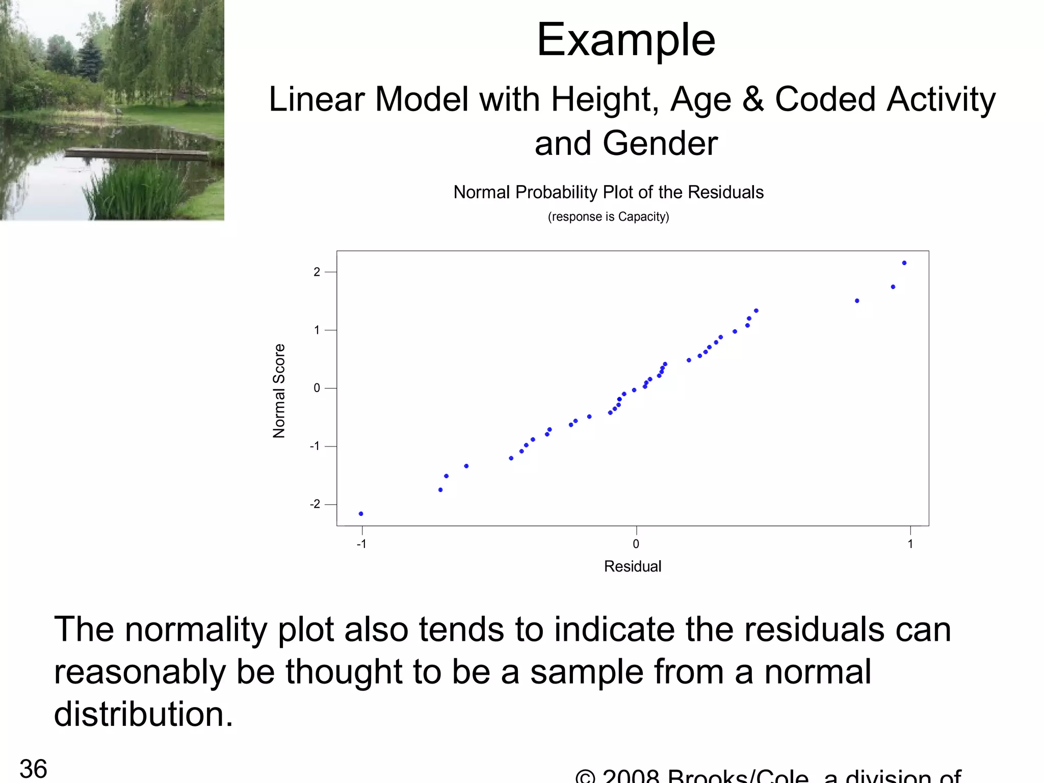
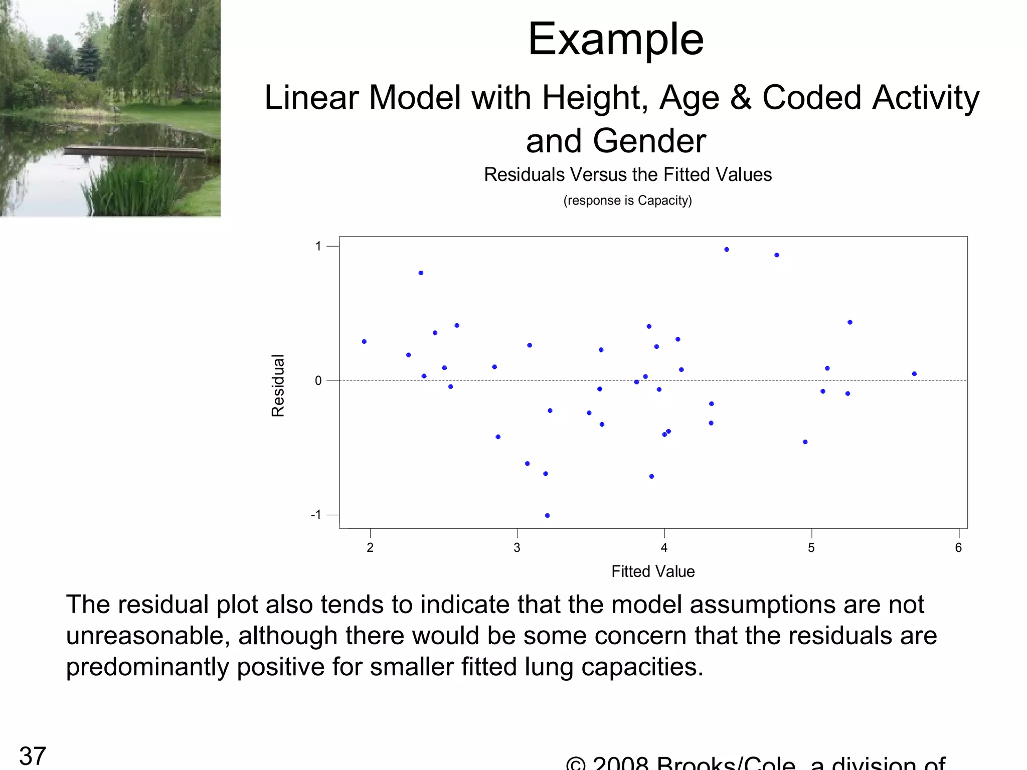
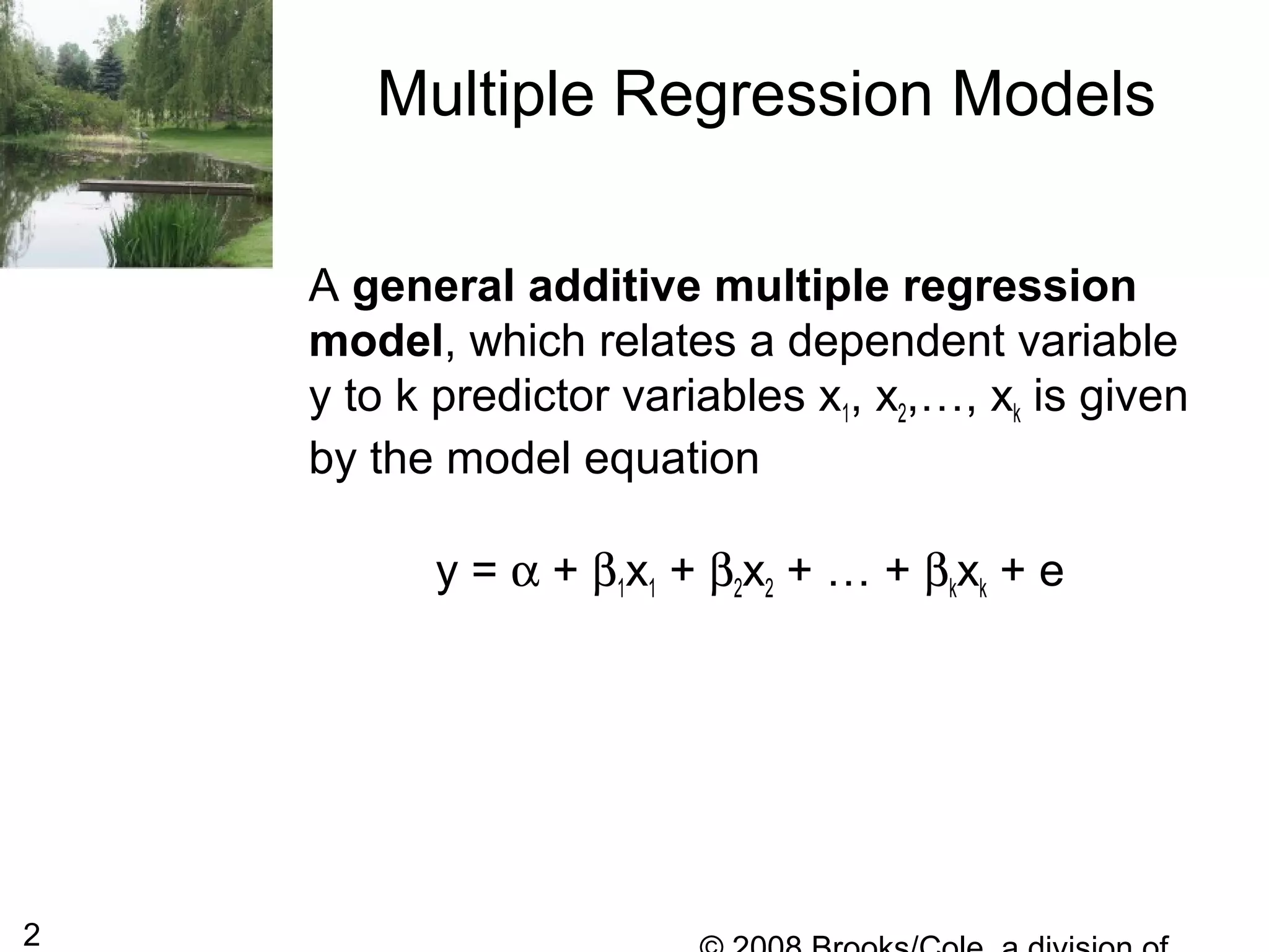
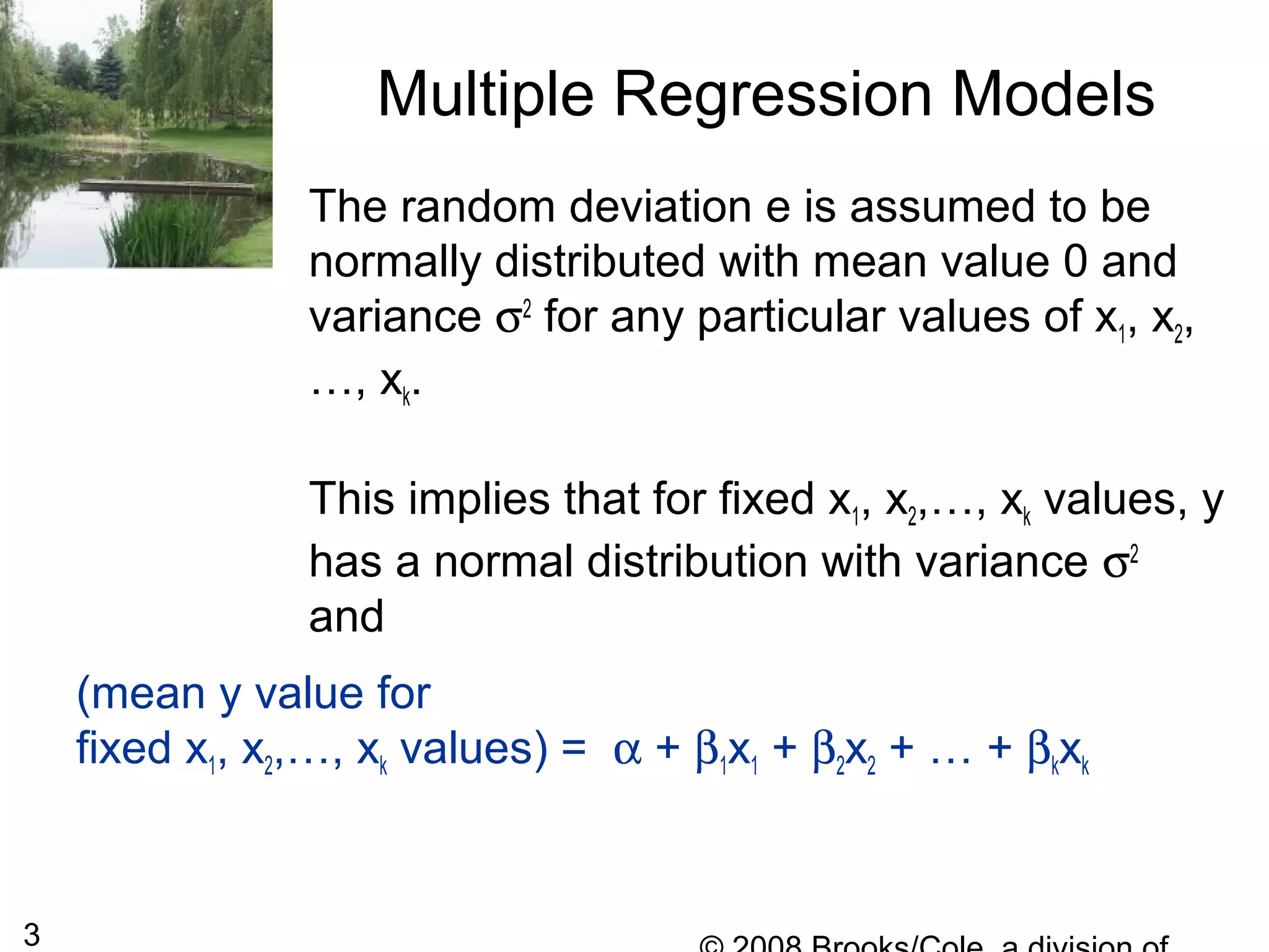
1. 1
Chapter 14
Multiple Regression Models

2. 2
A general additive multiple regression
model, which relates a dependent variable
y to k predictor variables x1, x2,…, xk is given
by the model equation
y = α + β1x1 + β2x2 + … + βkxk + e
Multiple Regression Models

3. 3
The random deviation e is assumed to be
normally distributed with mean value 0 and
variance σ2
for any particular values of x1, x2,
…, xk.
This implies that for fixed x1, x2,…, xk values, y
has a normal distribution with variance σ2
and
Multiple Regression Models
(mean y value for
fixed x1, x2,…, xk values) = α + β1x1 + β2x2 + … + βkxk

4. 4
The βi’s are called population regression
coefficients; each βi can be interpreted as
the true average change in y when the
predictor xi increases by 1 unit and the
values of all the other predictors remain
fixed.
Multiple Regression Models
The deterministic portion
α+ β1x1 + β2x2 + … + βkxk
is called the population regression function.

5. 5
The kth
degree polynomial regression
model
y = α + β1x + β2x2
+ … + βkxk
+ e
is a special case of the general multiple
regression model with x1 = x, x2 = x2
, … , xk
= xk
.
The population regression function
(mean value of y for fixed values of the
predictors) is
α + β1x + β2x2
+ … + βkxk
.
Polynomial Regression Models

6. 6
The most important special case other than
simple linear regression (k = 1) is the
quadratic regression model
y = α+ β1x + β2x2
.
This model replaces the line y = α+ βx with a
parabolic cure of mean values α + β1x + β2x2
.
If β2 > 0, the curve opens upward, whereas if
β2 < 0, the curve opens downward.
Polynomial Regression Models

7. 7
If the change in the mean y value
associated with a 1-unit increase in one
independent variable depends on the value
of a second independent variable, there is
interaction between these two variables.
When the variables are denoted by x1 and
x2, such interaction can be modeled by
including x1x2, the product of the variables
that interact, as a predictor variable.
Interaction

8. 8
Up to now, we have only considered the
inclusion of quantitative (numerical) predictor
variables in a multiple regression model.
Two other types are very common:
Dichotomous variable: One with just two
possible categories coded 0 and 1
Examples
 Gender {male, female}
 Marriage status {married, not-
married}
Qualitative Predictor Variables.

9. 9
Ordinal variables: Categorical variables
that have a natural ordering
 Activity level {light, moderate,
heavy} coded respectively as 1, 2
and 3
 Education level {none, elementary,
secondary, college, graduate}
coded respectively 1, 2, 3, 4, 5 (or
for that matter any 5 consecutive
integers}
Qualitative Predictor Variables.

10. 10
According to the principle of least squares,
the fit of a particular estimated regression
function a + b1x1 + b2x2 + … + bkxk to the
observed data is measured by the sum of
squared deviations between the observed y
values and the y values predicted by the
estimated function:
Σ[y –(a + b1x1 + b2x2 + … + bkxk )]2
Least Square Estimates
The least squares estimates of α, β1, β2,…, βk are
those values of a, b1, b2, … , bk that make this sum of
squared deviations as small as possible.

11. 11
Predicted Values & Residuals
Doing this successively for the remaining
observations yields the predicted values
(sometimes referred to as the fitted values or fits).
L2 3 ky ,y , ,yˆ ˆ ˆ
The first predicted value is obtained by
taking the values of the predictor variables
x1, x2,…, xk for the first sample observation
and substituting these values into the
estimated regression function.
1ˆy

12. 12
Predicted Values & Residuals
The residuals are then the differences
between the observed and predicted y
values.
− − −L1 1 2 2 k ky y ,y y , ,y yˆ ˆ ˆ

13. 13
Sums of Squares
The number of degrees of freedom associated with
SSResid is n - (k + 1), because k + 1 df are lost in
estimating the k + 1 coefficients α, β1, β2,…,βk.
The residual (or error) sum of sqyares,
SSResid, and total sum of squares,
SSTo, are given by
where is the mean of the y observations
in the sample.
( ) ( )
2 2
ˆSSResid= y-y SSTo= y-y∑ ∑
y

14. 14
Estimate for σ2
An estimate of the random deviation
variance σ2
is given by
and is the estimate of σ.
2
e
SSResid
s
n - (k + 1)
=
2
e es s=

15. 15
Coefficient of Multiple Determination, R2
The coefficient of multiple
determination, R2
, interpreted as the
proportion of variation in observed y values
that is explained by the fitted model, is
2 SSResid
R 1
SSTo
= −

16. 16
Adjusted R2
Generally, a model with large R2
and small
se are desirable. If a large number of
variables (relative to the number of data
points) is used those conditions may be
satisfied but the model will be unrealistic
and difficult to interpret.

17. 17
Adjusted R2
To sort out this problem, sometimes
computer packages compute a quantity
called the adjusted R2
,
2 n 1 SSResid
adjusted R 1
n (k 1) SSTo
− 
= −  − − 
Notice that when a large number of variables are
used to build the model, this value will be
substantially lower than R2
and give a better
indication of usability of the model.

18. F Distributions
F distributions are similar to a Chi-Square
distributions, but have two parameters, dfden and
dfnum.

19. 19
The F Test for Model Utility
The regression sum of squares
denoted by SSReg is defined by
SSREG = SSTo - SSresid

20. 20
The F Test for Model Utility
When all k βi’s are zero in the model
y = α + β1x1 + β2x2 + … + βkxk + e
And when the distribution of e is normal
with mean 0 and variance σ2
for any
particular values of x1, x2,…, xk, the statistic
has an F probability distribution based on k
numerator df and n - (K+ 1) denominator df
SSRegr
kF
SSResid
n (k 1)
=
− +

21. 21
The F Test for Utility of the Model
y = α + β1x1 + β2x2 + … + βkxk + e
Null hypothesis:
H0: β1 = β2 = … = βk =0
(There is no useful linear relationship
between y and any of the predictors.)
Alternate hypothesis:
Ha: At least one among β1, β2, … , βk is
not zero
(There is a useful linear relationship
between y and at least one of the
predictors.)

22. 22
The F Test for Utility of the Model
y = α + β1x1 + β2x2 + … + βkxk + e
Test statistic: SSRegr
kF
SSResid
n (k 1)
where SSreg = SST0 - SSresid.
=
− +
An alternate formula:
2
2
R
kF
(1 R )
n (k 1)
where SSreg = SST0 - SSresid.
=
−
− +

23. 23
The F Test Utility of the Model
y = α + β1x1 + β2x2 + … + βkxk + e
The test is upper-tailed, and the information
in the Table of Values that capture specified
upper-tail F curve areas is used to obtain a
bound or bounds on the P-value using
numerator df = k and denominator
df = n - (k + 1).
Assumptions: For any particular combination of
predictor variable values, the distribution of e, the
random deviation, is normal with mean 0 and
constant variance.

24. 24
Example
A number of years ago, a group of college
professors teaching statistics met at an NSF
program and put together a sample student
research project.
They attempted to create a model to explain lung
capacity in terms of a number of variables.
Specifically,
Numerical variables: height, age, weight, waist
Categorical variables: gender, activity level and
smoking status.

25. 25
Example
They managed to sample 41 subjects and
obtain/measure the variables.
There was some discussion and many felt
that the calculated variable (height)(waist)2
would be useful since it would likely be
proportional to the volume of the individual.
The initial regression analysis performed
with Minitab appears on the next slide.

26. 26
Example
Linear Model with All Numerical Variables
The regression equation is
Capacity = - 13.0 - 0.0158 Age + 0.232 Height - 0.00064
Weight - 0.0029 Chest
+ 0.101 Waist -0.000018 hw2
40 cases used 1 cases contain missing values
Predictor Coef SE Coef T P
Constant -13.016 2.865 -4.54 0.000
Age -0.015801 0.007847 -2.01 0.052
Height 0.23215 0.02895 8.02 0.000
Weight -0.000639 0.006542 -0.10 0.923
Chest -0.00294 0.06491 -0.05 0.964
Waist 0.10068 0.09427 1.07 0.293
hw2 -0.00001814 0.00001761 -1.03 0.310
S = 0.5260 R-Sq = 78.2% R-Sq(adj) = 74.2%

27. 27
Example
The only coefficient that appeared to be
significant and the 5% level was the height.
Since the P-value for the coefficient on the
age was very close to 5% (5.2%) it was
decided that a linear model with the two
independent variables height and age would
be calculated.
The resulting model is on the next slide.

28. 28
Example
Linear Model with variables: Height & Age
The regression equation is
Capacity = - 10.2 + 0.215 Height - 0.0133 Age
40 cases used 1 cases contain missing values
Predictor Coef SE Coef T P
Constant -10.217 1.272 -8.03 0.000
Height 0.21481 0.01921 11.18 0.000
Age -0.013322 0.005861 -2.27 0.029
S = 0.5073 R-Sq = 77.2% R-Sq(adj) = 76.0%
Notice that even though the R2
value decreases slightly, the
adjusted R2
value actually increases. Also note that the
coefficient on Age is now significant at 5%.

29. 29
Example
In an attempt to determine if incorporating
the categorical variables into the model
would significantly enhance the it.
Gender was coded as an indicator variable
(male = 0 and female = 1),
Smoking was coded as an indicator variable
(No = 0 and Yes = 1), and
Activity level (light, moderate, heavy) was
coded respectively as 1, 2 and 3.
The resulting Minitab output is given on the
next slide.

30. 30
Example
Linear Model with categorical variables added
The regression equation is
Capacity = - 7.58 + 0.171 Height - 0.0113 Age - 0.383 C-Gender
+ 0.260 C-Activity - 0.289 C-Smoke
37 cases used 4 cases contain missing values
Predictor Coef SE Coef T P
Constant -7.584 2.005 -3.78 0.001
Height 0.17076 0.02919 5.85 0.000
Age -0.011261 0.005908 -1.91 0.066
C-Gender -0.3827 0.2505 -1.53 0.137
C-Activi 0.2600 0.1210 2.15 0.040
C-Smoke -0.2885 0.2126 -1.36 0.185
S = 0.4596 R-Sq = 84.2% R-Sq(adj) = 81.7%

31. 31
Example
It was noted that coefficient for the coded
indicator variables gender and smoking
were not significant, but after considerable
discussion, the group felt that a number of
the variables were related.
This, the group felt, was confounding the study. In an
attempt to determine a reasonable optimal subgroup of
the variables to keep in the study, it was noted that a
number of the variables were highly related. Since the
study was small, a stepwise regression was run and the
variables, Height, Age, Coded Activity, Coded Gender
were kept and the following model was obtained.

32. 32
Example
Linear Model with Height, Age & Coded Activity
and Gender
The regression equation is
Capacity = - 6.93 + 0.161 Height - 0.0137 Age
+ 0.302 C-Activity - 0.466 C-Gender
40 cases used 1 cases contain missing values
Predictor Coef SE Coef T P
Constant -6.929 1.708 -4.06 0.000
Height 0.16079 0.02454 6.55 0.000
Age -0.013744 0.005404 -2.54 0.016
C-Activi 0.3025 0.1133 2.67 0.011
C-Gender -0.4658 0.2082 -2.24 0.032
S = 0.4477 R-Sq = 83.2% R-Sq(adj) = 81.3%

33. 33
Example
Linear Model with Height, Age & Coded Activity
and Gender
Analysis of Variance
Source DF SS MS F P
Regression 4 34.8249 8.7062 43.44 0.000
Residual Error 35 7.0151 0.2004
Total 39 41.8399
Source DF Seq SS
Height 1 30.9878
Age 1 1.3296
C-Activi 1 1.5041
C-Gender 1 1.0034
Unusual Observations
Obs Height Capacity Fit SE Fit Residual St Resid
4 66.0 2.2000 3.2039 0.1352 -1.0039 -2.35R
23 74.0 5.7000 4.7635 0.2048 0.9365 2.35R
39 70.0 5.4000 4.4228 0.1064 0.9772 2.25R
R denotes an observation with a large standardized residual
The rest of the Minitab output is given below.

34. 34
Example
Linear Model with Height, Age & Coded Activity
and Gender
All of the coefficients in this model were
significant at the 5% level and the R2
and
adjusted R2
were both fairly large.
This appeared to be a reasonable model for
describing lung capacity even though the
study was limited by sample size, and
measurement limitations due to antique
equipment.
Minitab identified 3 outliers (because the standardized
residuals were unusually large.
Various plots of the standardized residuals are produced
on the next few slides with comments

35. 35
Example
Linear Model with Height, Age & Coded Activity
and Gender
The histogram of the residuals appears to be consistent with
the assumption that the residuals are a sample from a
normal distribution.
1.00.80.60.40.20.0-0.2-0.4-0.6-0.8-1.0
10
5
0
Residual
Frequency
Histogram of the Residuals
(response is Capacity)

36. 36
Example
Linear Model with Height, Age & Coded Activity
and Gender
The normality plot also tends to indicate the residuals can
reasonably be thought to be a sample from a normal
distribution.
10-1
2
1
0
-1
-2
NormalScore
Residual
Normal Probability Plot of the Residuals
(response is Capacity)

37. 37
Example
Linear Model with Height, Age & Coded Activity
and Gender
The residual plot also tends to indicate that the model assumptions are not
unreasonable, although there would be some concern that the residuals are
predominantly positive for smaller fitted lung capacities.
65432
1
0
-1
Fitted Value
Residual
Residuals Versus the Fitted Values
(response is Capacity)