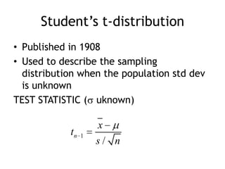
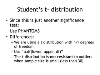
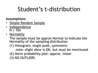
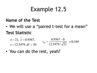
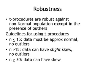
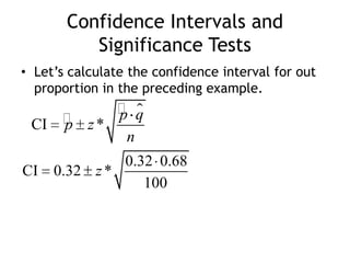
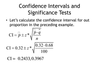
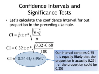
This document discusses significance tests for population means and proportions using Student's t-distribution and the normal distribution. It provides examples of hypothesis testing for a population mean using a paired t-test and for a population proportion using a single-sample z-test. It also discusses the assumptions, test statistics, and interpretations for these tests. Confidence intervals are presented as complementary to significance tests for estimating population parameters.

1. Chapter 12Significance Tests in Practice

2. 12.1 Tests about Population Mean

3. Student’s t-distributionPublished in 1908Used to describe the sampling distribution when the population std dev is unknownTEST STATISTIC ( uknown)

4. Student’s t- distributionSince this is just another significance test: Use PHANTOMSDifferences:We are using a t distribution with n-1 degrees of freedomUse “tcdf(lower, upper, df)”The t-distribution is not resistant to outliers when sample size is small (less than 30)

5. Student’s t-distributionAssumptionsSimple Random SampleIndependenceN > 10nNormalityThe sample must be approx Normal to indicate the Normality of the sampling distribution(1) Histogram: single peak, symmetric note: slight skew is OK, but must be mentioned(2) Norm probability plot: approx. linear(3) NO OUTLIERS

6. Example 12.2 Tasters use a “sweetness scale” of 1 to 10. Cola is rated before and after a month of storage in high temperature. The differences are shown below. The bigger the difference, the greater the loss of sweetness. Does the data indicate that sweetness was lost after the storage interval? 2.0, 0.4, 0.7, 2.0, -0.4, 2.2, -1.3, 1.2, 1.1, 2.3

7. Example 12.2ParameterLet  = the population mean sweetness lost after a month of storage at high temperatureLet xbar = the sample (n=10) sweetness loss after a month of storage at high temperatures

8. Example 12.2HypothesesH0:  = 0This indicates that there is no sweetness loss Ha:  > 0This indicates that there is sweetness loss

9. Example 12.2AssumptionsSimple Random SampleWe are not told that our data represents an SRS. We must check that this sample is an SRS (or acts like an SRS) and proceed.IndependenceWe can be assured that the population of cola is greater than 10(10) = 100

10. Example 12.2Assumptions (cont.)Normality Our histogram is single peaked with a slight left skew The Normal probability plot is approximately linear There are no outliers

11. Example 12.2Test StatisticP-value

12. Example 12.2Test StatisticP-value

13. Example 12.2Test StatisticP-value

14. Example 12.2Test StatisticP-value

15. Example 12.2Test StatisticP-value

16. Example 12.2Test StatisticP-value

17. Example 12.2Test StatisticP-value

18. Example 12.2Make a decisionWe are going to “reject” (our p-value is small)SummarizeApproximately 1% of the time, a sample of size 10 will produce a mean sweetness loss of at least 1.02.Since the p-value is smaller than a presumed  = 0.05, we reject the null hypothesis.We have evidence to conclude that the mean sweetness loss greater than 0. Our new estimate for the average sweetness loss is 1.02.

19. Paired t-testsWhen a sample is produced using a matched pair design, the data used in the significance test is the difference of the two measurementsSome typical examples of a paired t-test would be a “pre-test and post-test” as well as the previous example.The important thing here is to recognize the matched pair design and to work of the difference of the scores (and not the scores themselves)

20. Example 12.5

21. Example 12.5 We will work through the first few steps and leave the rest for you on your own.Parameter = the population difference in average time to complete the maze xbar = the sample (n = 21) difference in average time to complete the maze

22. Example 12.5HypothesesH0:  = 0Ha:  > 0(the scented mask decreases average time to complete maze)Remember: we are looking at the “difference” column only!

23. Example 12.5AssumptionsSimple Random SampleThe data comes from a randomized matched pair design; we will have to assume that this is an SRS of the population and proceed with the testIndependenceWe must assume that the population is greater than 10(21) = 210 and that the scented and unscented trails are independent; we will proceed as though this condition is satisfied

24. Example 12.5Assumptions (cont.)Normality Our histogram is single peaked with a slight right skew The Normal probability plot is approximately linear There are no outliers

25. Example 12.5Name of the TestWe will use a “paired t-test for a mean”Test StatisticYou can do the rest, yeah?

26. Robustnesst-procedures are robust against non-Normal population except in the presence of outliersGuidelines for using t-proceduresn < 15: data must be approx normal,no outliersn >15: data can have slight skew, no outliersn > 30: data can have skew

27. Assignment 12.1Page 745 #1, 3, 6, 9, 10, 12, 16, 20

28. 12.2 Tests about a Population Proportion

29. z-tests for proportionAgain, we have introduced most of the material- this is just another significance test.Unlike tests for means, tests for proportions will always be a z-testWe will review some of the key information:

30. Assumptions for proportionsSimple Random SampleIndependenceN > 10nNormality (of sampling distribution)np> 10 and nq>10remember that this is just the number of responses

31. Test Statistic for proportionsIf H0: p = p0

32. Example 12.8 A random sample of 100 workers from a large chain restaurant were asked whether or not work stress had a negative impact on their personal lives. Thirty-two of them responded “No.” A large national survey reported that 25% of restaurant workers did not feel that stress exerted a negative impact. Does this large chain restaurant have the same work stress as the nation?

33. Example 12.8We are going to use the national survey as our known population mean.Parameterp = the national proportion of restaurant workers who feel as though work stress has a negative impact on their personal lives.p-hat = the proportion of the sample of 100 workers who feel as though work stress has a negative impact on their personal lives.

34. Example 12.8Hypotheses H0: p = 0.25 Ha: p  0.25AssumptionsSimple Random Sample We are told that our sample is from a random sample. We will treat this as an SRS.Independence Although we are not told, we will make the assumption that there are more than 10(100) = 1000 workers for this national chainNormalitynp = 38 >10 and nq = 62 > 10Our sampling distribution is approximately Normal

35. Example 12.8Name of Test We will conduct a 1-proportion z-test (Note that this will be a two-tailed test)Test Statistic

36. Example 12.8PvalueDecision

37. Example 12.8PvalueDecision

38. Example 12.8PvalueDecision

39. Example 12.8PvalueDecision

40. Example 12.8PvalueDecisionFail to reject

41. Example 12.8Summarize Approximately 11% of the time, a sample of size 100 will produce a proportion at least as extreme 0.38. Since this is not less than a presumed  = 0.05, we will fail to reject the H0. We do not have enough evidence to conclude that the proportion of workers of this national chain who feel that work stress affects their personal lives is not 0.25.

42. PowerThe preceding example should make you feel a bit uncomfortable: that p-value was not large. We don’t really expect the average to be exactly equal to the national average! Most likely, the restaurant’s proportion was not that different from the national average: maybe just a few percentage points greater. Our test didn’t have enough power to detect the difference between the two proportions!

43. Confidence Intervals and Significance TestsLet’s calculate the confidence interval for out proportion in the preceding example.

44. Confidence Intervals and Significance TestsLet’s calculate the confidence interval for out proportion in the preceding example.

45. Confidence Intervals and Significance TestsLet’s calculate the confidence interval for out proportion in the preceding example.Notice that the Conf. Int.uses p-hat and q-hat for the Standard Error

46. Confidence Intervals and Significance TestsLet’s calculate the confidence interval for out proportion in the preceding example.

47. Confidence Intervals and Significance TestsLet’s calculate the confidence interval for out proportion in the preceding example.

48. Confidence Intervals and Significance TestsLet’s calculate the confidence interval for out proportion in the preceding example.Our interval contains 0.25It is equally likely that theproportion is actually 0.25!i.e. the proportion could be0.25!

49. Calculator Usage As you may have already noticed, the TI calculators automate many of these calculations. Of course, this does not excuse you from writing out the PHANTOMS or PANIC procedures, or even showing your calculations!

50. Calculator Usage

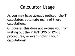
51. Calculator UsageTI83/84: Since these functions are menu driven we will just list the tests and their usage [STAT] -> “TESTS”Z-Test = one or two tailed z test for meanT-Test = one or two tail t-test for means1-PropZTest = one or two tail test for proportionsZInterval = confidence interval for mean (-known)Tinterval = confidence interval for mean (-unknown)1-PropZInt = confidence interval for proportions