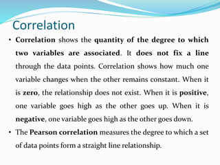
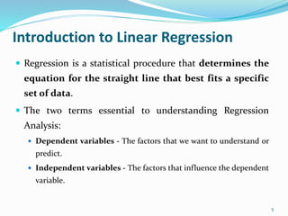
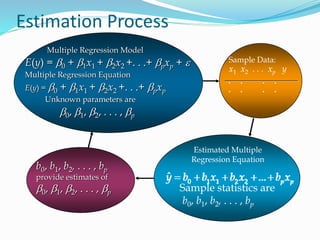
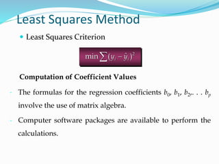
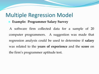
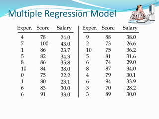
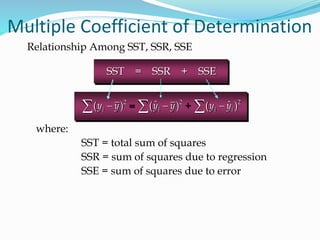
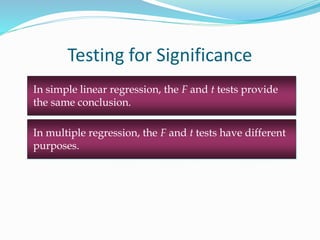
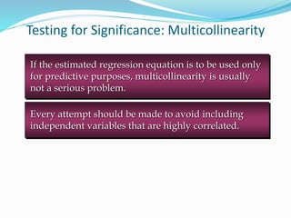
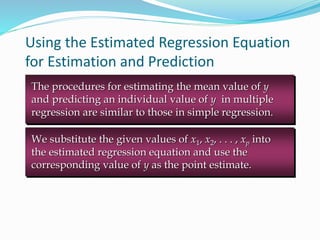
The document discusses the transformation of data into information and knowledge, highlighting the concepts of correlation and regression. It explains linear regression methods, including least squares regression, and provides examples and Python code for implementation using libraries such as NumPy and scikit-learn. Additionally, it touches on multiple regression, the interpretation of coefficients, goodness-of-fit measures like R-squared, and significance testing methods such as t-tests and F-tests.


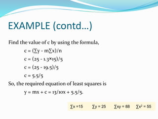
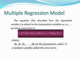
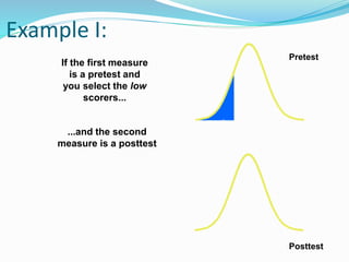
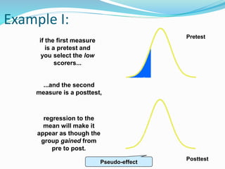
![EXAMPLE (contd…)
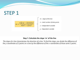
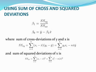
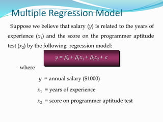
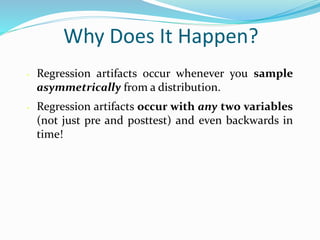
Find the value of m by using the formula,
m = (n∑xy - ∑y∑x)/n∑x2 - (∑x)2
m = [(5×88) - (15×25)]/(5×55) - (15)2
m = (440 - 375)/(275 - 225)
m = 65/50 = 13/10
∑x =15 ∑y = 25 ∑xy = 88 ∑x2 = 55](https://image.slidesharecdn.com/ds-regression-220812044010-7b26c678/85/Regression-14-320.jpg)
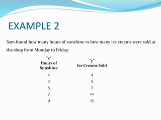
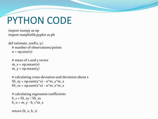
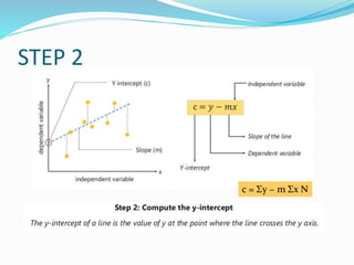
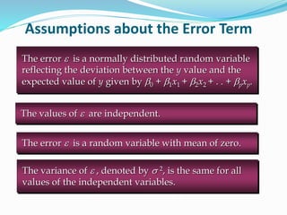
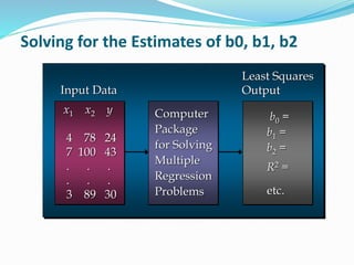
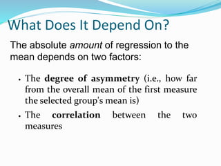
![PYTHON CODE
def plot_regression_line(x, y, b):
# plotting the actual points as scatter plot
plt.scatter(x, y, color = "m",
marker = "o", s = 30)
# predicted response vector
y_pred = b[0] + b[1]*x
# plotting the regression line
plt.plot(x, y_pred, color = "g")
# putting labels
plt.xlabel('x')
plt.ylabel('y')
# function to show plot
plt.show()](https://image.slidesharecdn.com/ds-regression-220812044010-7b26c678/85/Regression-21-320.jpg)
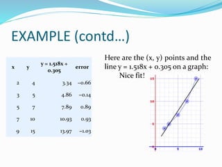
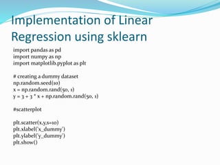
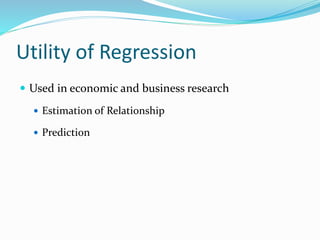
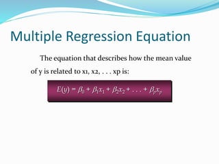
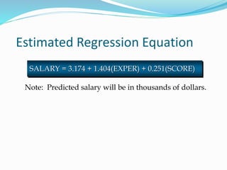
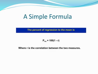
![PYTHON CODE
def main():
# observations / data
x = np.array([0, 1, 2, 3, 4, 5, 6, 7, 8, 9])
y = np.array([1, 3, 2, 5, 7, 8, 8, 9, 10, 12])
# estimating coefficients
b = estimate_coef(x, y)
print("Estimated coefficients:nb_0 = {}
nb_1 = {}".format(b[0], b[1]))
# plotting regression line
plot_regression_line(x, y, b)
if __name__ == "__main__":
main()
OUTPUT:
Estimated coefficients:
b_0 = -0.0586206896552
b_1 = 1.45747126437](https://image.slidesharecdn.com/ds-regression-220812044010-7b26c678/85/Regression-22-320.jpg)
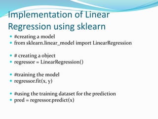
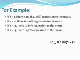
![Implementation of Linear
Regression using sklearn
#model performance
from sklearn.metrics import r2_score, mean_squared_error
mse = mean_squared_error(y, pred)
r2 = r2_score(y, pred)#Best fit lineplt.scatter(x, y)
plt.plot(x, pred, color = 'Black', marker = 'o')
#Results
print("Mean Squared Error : ", mse)
print("R-Squared :" , r2)
print("Y-intercept :" , regressor.intercept_)
print("Slope :" , regressor.coef_)
OUTPUT:
R-Squared : 0.9068822972556425
Y-intercept : [3.41354381]
Slope : [[3.11024701]]](https://image.slidesharecdn.com/ds-regression-220812044010-7b26c678/85/Regression-25-320.jpg)

![Interpret R-squared in Regression
Analysis (contd…)
We need to calculate two things:
var(avg) = ∑(yi – Ӯ)2
var(model) = ∑(yi – ŷ)2
R2 = 1 – [var(model)/var(avg)]
= 1 -[∑(yi – ŷ)2/∑(yi – Ӯ)2]](https://image.slidesharecdn.com/ds-regression-220812044010-7b26c678/85/Regression-46-320.jpg)


![Getting Started with Apache Spark: Big Data Made Simple [Free Meetup]](https://cdn.slidesharecdn.com/ss_thumbnails/apachesparkgettingstarted-260203175547-8361bcc3-thumbnail.jpg?width=640&height=640&fit=bounds)


