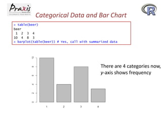
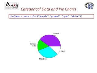
The document provides an introduction to basic operations and functions in R including: - Creating and manipulating numeric vectors using functions like c(), mean(), max(), and indexing - Creating and manipulating character vectors - Using positive and negative indexing to subset vectors - Appending values to existing vectors - Creating and summarizing categorical data using factors and functions like table() - 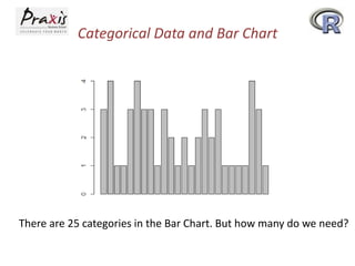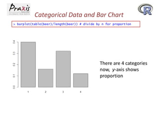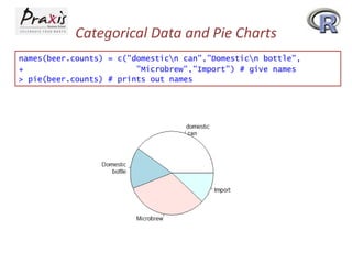Creating bar plots and pie charts to visualize categorical data - 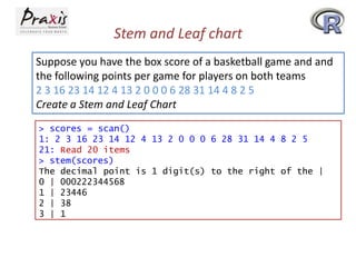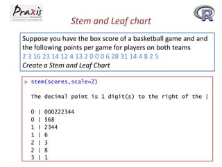Creating a stem-and-leaf plot to visualize a distribution

1. Let’s start with R
> typos = c(2,3,0,3,1,0,0,1)
> typos
[1] 2 3 0 3 1 0 0 1
> mean(typos)
[1] 1.25
> median(typos)
[1] 1
> var(typos)
[1] 1.642857
•
•
•
•
“typos” represent number of typing errors on different pages
Note that each command is stored in history
You can use UP arrow key to retrieve your previous command
You have started using built-in functions

2. Let’s start with R
> typos.draft1 = c(2,3,0,3,1,0,0,1)
> typos.draft2 = c(0,3,0,3,1,0,0,1)
> typos.draft1
[1] 2 3 0 3 1 0 0 1
> typos.draft2
[1] 0 3 0 3 1 0 0 1
• Note the two different object names for two drafts
• Period has been used as punctuation in object names
• Both the object names represent a vector

3. Let’s start with R
> typos.draft1 = c(2,3,0,3,1,0,0,1)
> typos.draft2 = typos.draft1 # make a copy
> typos.draft2[1] = 0 # assign the first page 0 typing error
> typos.draft2
[1] 0 3 0 3 1 0 0 1
• Note how we have created the same typos.draft2
• “#” has been used for comments
• ‘()’ are for functions and ‘*+’ are for vectors

4. Now try and check ….
> typos.draft2 # print out the value
[1] 0 3 0 3 1 0 0 1
> typos.draft2[2] # print 2nd pages' value
[1] 3
> typos.draft2[4] # 4th page
[1] 3
> typos.draft2[-4] # all but the 4th page
[1] 0 3 0 1 0 0 1
> typos.draft2[c(1,2,3)] # print values for 1st, 2nd and 3rd.
[1] 0 3 0
• Note the output of the last command. This is called Slicing.

5. Numeric Vector
• Simplest data structure in R
• To set up a numeric vector named x assign values :
> x <- c(23.0,17.0,12.5,11.0,17.0,12.0,14.5,9.0,11.0)
> x
[1] 23.0 17.0 12.5 11.0 17.0 12.0 14.5 9.0 11.0
Or
> assign ("x", c(23.0,17.0,12.5,11.0,17.0,12.0,14.5,9.0,11.0))
> x
[1] 23.0 17.0 12.5 11.0 17.0 12.0 14.5 9.0 11.0

6. Numeric Vector
or
> rm(x)
> c(23.0,17.0,12.5,11.0,17.0,12.0,14.5,9.0,11.0) -> x
> x
[1] 23.0 17.0 12.5 11.0 17.0 12.0 14.5 9.0 11.0
Look at the next assignment
> y <- c(x,0,1)
> y
[1] 23.0 17.0 12.5 11.0 17.0 12.0 14.5
9.0 11.0
0.0
1.0
A vector y has been created with a copy of x with a zero and one
at the end.

7. Character Vector
A character vector is a set of text values
> weekdays <- c("Sun","Mon","Tues","Wed","Thurs","Fri","Sat")
> weekdays
[1] "Sun"
"Mon"
"Tues" "Wed"
"Thurs" "Fri"
"Sat"

8. Positive Index
• A positive index can appended in square brackets to the name
of a vector
• It helps to select subsets of the elements of a vector
> x[2]
[1] 17
> x[1:9]
[1] 23.0 17.0 12.5 11.0 17.0 12.0 14.5
> x[3:7]
[1] 12.5 11.0 17.0 12.0 14.5
> x[c(2,5,7)]
[1] 17.0 17.0 14.5
9.0 11.0
• How do you find the number of elements in a vector?
> X
[1] 23.0 17.0 12.5 11.0 17.0 12.0 14.5
>length(x)
[1] 9
9.0 11.0

9. Negative Index
• A negative index specifies the element(s) to be excluded
rather than included
> y<-x[-2] #Include all but the second element
> y
[1] 23.0 12.5 11.0 17.0 12.0 14.5 9.0 11.0
> x
[1] 23.0 17.0 12.5 11.0 17.0 12.0 14.5 9.0 11.0
• How do you exclude more than one element?
> X
[1] 23.0 17.0 12.5 11.0 17.0 12.0 14.5 9.0 11.0
> y<-x[-(2:4)]
> y
[1] 23.0 17.0 12.0 14.5 9.0 11.0
> y<-x[-(c((2:4),9))] #exclude 2nd to 4th, and 9th elements
> y
[1] 23.0 17.0 12.0 14.5 9.0

10. Now try and check ….
> typos.draft2
# show all the values
[1] 0 3 0 3 1 0 0 1
> max(typos.draft2) # what are worst pages?
[1] 3
> typos.draft2 == 3 # Where are they?
[1] FALSE TRUE FALSE TRUE FALSE FALSE FALSE FALSE
• Note the use of ‘==‘ for comparing
• But how do we get the indices (pages) having 3 typos?
> which(typos.draft2 == 3)
[1] 2 4
• You only get the index of the elements

11. Now try and check ….
> n = length(typos.draft2) # how many pages
> pages = 1:n # how we get the page numbers
> pages # pages is simply 1 to number of pages
[1] 1 2 3 4 5 6 7 8
> pages[typos.draft2 == 3] # logical extraction. Very useful
[1] 2 4
The idea is to create a new vector 1, 2, 3, …. keeping track of page
numbers and then slicing off ones for which typos.draft2===3

12. Now try and check ….
> sum(typos.draft2) # How many typos?
[1] 8
> sum(typos.draft2>0) # How many pages with typos?
[1] 4
> typos.draft1 - typos.draft2 # difference between the two
[1] 2 0 0 0 0 0 0 0
Well Done … Great!!

13. Now try and check ….
Suppose the daily closing price of your favourite stock for two weeks is
45,43,46,48,51,46,50,47,46,45
How do you keep track of this?
> x = c(45,43,46,48,51,46,50,47,46,45)
> x
[1] 45 43 46 48 51 46 50 47 46 45
> mean(x) # the mean
[1] 46.7
> median(x) # the median
[1] 46
> max(x) # the maximum or largest value
[1] 51
> min(x) # the minimum value
[1] 43
Hope you are enjoying many interesting functions ………

14. Now try and check ….
Let’s add the next two weeks worth of data to x. This was
48,49,51,50,49,41,40,38,35,40
> x = c(x,48,49,51,50,49) #
> length(x) # how long is x
[1] 15
> x[16] = 41 # add value to
> x[17:20] = c(40,38,35,40)
> x
[1] 45 43 46 48 51 46 50 47
append values to x
now (it was 10)
a specified index which is 16
# add to many specified indices
46 45 48 49 51 50 49 41 40 38 35 40
We did three different things to add to a vector.
• We used the c (combine) operator to combine the previous
value of x with the next week's numbers.
• We then assigned directly to the 16th index.
• Finally, we assigned to a slice of indices.

15. Now try and check ….
Suppose we want a 5-day moving average
> day<-5
> mean(x[day:(day+4)])
[1] 48
> day:(day+4)
[1] 5 6 7 8 9
How do you get running maximum or minimum till date?
> cummax(x) # running
[1] 45 45 46 48 51 51
> cummin(x) # running
[1] 45 43 43 43 43 43
maximum
51 51 51 51 51 51 51 51 51 51 51 51 51 51
minimum
43 43 43 43 43 43 43 43 43 41 40 38 35 35

16. Self-test
Suppose you keep track of your mileage each time you fill up. At
your last 8 fill-ups the mileage was
65311 65624 65908 66219 66499 66821 67145 67447
Enter these numbers into R. Use the function ‘diff’ on the data.
What does it give?
Use the max function to find the maximum number of miles
between fill-ups, the mean function to find the average number
of miles and the min function to get the minimum number of
miles.

17. Self-test
Suppose you track your commute times for two weeks (10 days)
and you find the following times in minutes
17 16 20 24 22 15 21 15 17 22
Enter this into R. Use the function max to find the longest
commute time, the function mean to find the average and the
function min to find the minimum.
The 24 was a mistake. It should have been 18. How can you fix
this? Do so, and then find the new average.
How many times was your commute 20 minutes or more? To
answer this you can try (if you call your numbers commutes)
> sum( commutes >= 20)
What do you get? What percent of your commutes are less than
17 minutes? How can you answer this with R?

18. Categorical Data
A survey asks people if they smoke or not.
The data is Yes, No, No, Yes, Yes
We can enter this into R with the c() command, and summarize
with the table command as
> x=c("Yes","No","No","Yes","Yes")
> table(x)
x
No Yes
2
3
The table command simply adds up the frequency of each
unique value of the data.

19. Categorical Data : Factor
Categorical data is often used to classify data into various levels
or factors. To make a factor is easy with the command factor or
as.factor.
> x #Print the values in x
[1] "Yes" "No" "No" "Yes" "Yes"
> factor(x) # print out value in factor(x)
[1] Yes No No Yes Yes
Levels: No Yes
Note that levels have been printed.

20. Categorical Data and Bar Chart
A bar chart draws a bar with a height proportional to the count in
the table. The height could be given by the frequency, or the
proportion.
Suppose, a group of 25 people are surveyed as to their beerdrinking preference. The categories were (1) Domestic
can, (2) Domestic bottle, (3) Microbrew and (4) import. The raw
data is
3411343313212123231111431
> beer = scan()
1: 3 4 1 1 3 4 3 3 1 3 2 1 2 1 2 3 2 3 1 1 1 1 4 3 1
26:
Read 25 items
> barplot(beer) # this isn't correct

21. Categorical Data and Bar Chart
There are 25 categories in the Bar Chart. But how many do we need?

22. Categorical Data and Bar Chart
> table(beer)
beer
1 2 3 4
10 4 8 3
> barplot(table(beer)) # Yes, call with summarized data
There are 4 categories now,
y-axis shows frequency

23. Categorical Data and Bar Chart
> barplot(table(beer)/length(beer)) # divide by n for proportion
There are 4 categories
now, y-axis shows
proportion

24. Categorical Data and Pie Charts
> beer.counts = table(beer) # store the table result
> pie(beer.counts) # first pie -- kind of dull

25. Categorical Data and Pie Charts
names(beer.counts) = c("domesticn can","Domesticn bottle",
+
"Microbrew","Import") # give names
> pie(beer.counts) # prints out names

26. Categorical Data and Pie Charts
pie(beer.counts,col=c("purple","green2","cyan","white"))

27. Stem and Leaf chart
Suppose you have the box score of a basketball game and and
the following points per game for players on both teams
2 3 16 23 14 12 4 13 2 0 0 0 6 28 31 14 4 8 2 5
Create a Stem and Leaf Chart
> scores = scan()
1: 2 3 16 23 14 12 4 13 2 0 0 0 6 28 31 14 4 8 2 5
21: Read 20 items
> stem(scores)
The decimal point is 1 digit(s) to the right of the |
0 | 000222344568
1 | 23446
2 | 38
3 | 1

28. Stem and Leaf chart
Suppose you have the box score of a basketball game and and
the following points per game for players on both teams
2 3 16 23 14 12 4 13 2 0 0 0 6 28 31 14 4 8 2 5
Create a Stem and Leaf Chart
> stem(scores,scale=2)
The decimal point is 1 digit(s) to the right of the |
0
0
1
1
2
2
3
|
|
|
|
|
|
|
000222344
568
2344
6
3
8
1

29. Making numeric data categorical
Suppose, CEO yearly compensations are sampled and the
following are found (in millions).
12 0.4 5 2 50 8 3 1 4 0.25
And we want to break that data into the intervals [0; 1]; (1; 5];
(5; 50] and name the same.
> sals = c(12, .4, 5, 2, 50, 8, 3, 1, 4, .25) # enter data
> cats = cut(sals,breaks=c(0,1,5,max(sals))) # specify the breaks
> cats # view the values
[1] (5,50] (0,1] (1,5] (1,5] (5,50] (5,50] (1,5] (0,1] (1,5]
Levels: (0,1] (1,5] (5,50]
> levels(cats) = c("poor","rich","rolling in it") # change labels
> table(cats)
cats
poor
rich rolling in it
3
4
3
(0,1]