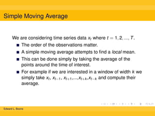
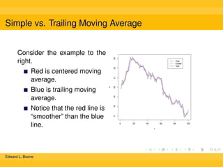
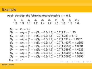
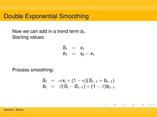
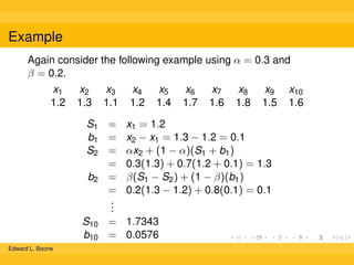
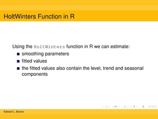
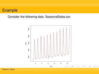
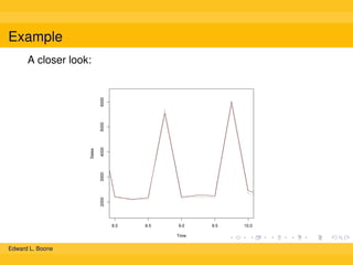
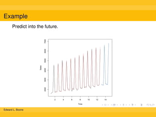
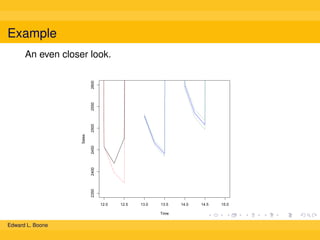
Moving Average Methods
Edward L. Boone
Department of Statistical Sciences and Operations Research
Virginia Commonwealth University

November 11, 2013

Edward L. Boone
Simple Moving Average

We are considering time series data xt where t = 1, 2, ..., T .
The order of the observations matter.
A simple moving average attempts to find a local mean.
This can be done simply by taking the average of the
points around the time of interest.
For example if we are interested in a window of width k we
simply take xt , xt−1 , xt+1 ,...,xt+k ,xt−k and compute their
average.

Edward L. Boone
Example
Consider the following example:
x1
1.2

x2
1.3

x3
1.1

x4
1.2

x5
1.4

x6
1.7

x7
1.6

x8
1.8

x9
1.5

x10
1.6

If we want the moving average at time t = 3 with window 2.
¯
x3,2 =

x1 + x2 + x3 + x4 + x5
1.2 + 1.3 + 1.1 + 1.2 + 1.4
=
= 1.24
5
5

If we want the moving average at time t = 7 with window 2.
¯
x7,2 =

x5 + x6 + x7 + x8 + x9
1.4 + 1.7 + 1.6 + 1.8 + 1.5
=
= 1.6
5
5

Notice that the “local” means are not similar.
Edward L. Boone
Trailing Moving Average
The problem with a standard moving average is that for the
mean at time t we need to know t + 1, t + 2,...,t + k , which is in
the future.
In many useful cases we don’t know the future.
We want to just use past values.
This leads to the idea of the trailing moving average.
Only take the average of xt−k , xt−k +1 ,...x1 , xt .
¯
xt,k =

Edward L. Boone

1
k

t

xt
i=t−k
Example
Again consider the following example.
x1
1.2

x2
1.3

x3
1.1

x4
1.2

x5
1.4

x6
1.7

x7
1.6

x8
1.8

x9
1.5

Trailing moving average with window k = 2
¯
x3,2 =

1.3 + 1.1 + 1.2
x2 + x3 + x4
=
= 1.2
3
3
.
.
.
x5 + x6 + x7
1.4 + 1.7 + 1.6
¯
=
=
= 1.56
3
3

¯
x4,2 =

¯
x7,2
Edward L. Boone

x1 + x2 + x3
1.2 + 1.3 + 1.1
=
= 1.2
3
3

x10
1.6
Simple vs. Trailing Moving Average

There are some issues that we will have to confront with all
time series methods.
How to handle the starting values?
Outliers?
Gaps?
Prediction?
Some of these are easier to deal with than others.

Edward L. Boone
Simple vs. Trailing Moving Average

23

Consider the example to the
right.

Edward L. Boone

22
x

20
19
18
17

Notice that the red line is
“smoother” than the blue
line.

21

Red is centered moving
average.
Blue is trailing moving
average.

True
Center
Trail

0

20

40

60
t

80

100
Issues with Moving Averages

Problems with simple moving average techniques.
In the previous methods, all observations in window get the
same weight.
We may wish to downweight observations as they get
farther in the past and always use all observations.
Gaps?
Prediction?
Some of these are easier to deal with than others.

Edward L. Boone
Exponentially Weighted Moving Average
A “simple” way to address the weighting problem is using a
weighted moving average.
There are several versions of these.
Each attempts to model the components of a time series
dataset.
If we just want to model the level then the Exponentially
Weighted Moving Average may be reasonable.
S1 = x1
St = αxt + (1 − α)St−1
These downweight the previous observations but still use
all observations.
Edward L. Boone
Example
Again consider the following example using α = 0.3.
x1
1.2
S1
S2
S3
S4
S5
S6
S7
S8
S9
S10
Edward L. Boone

=
=
=
=
=
=
=
=
=
=

x2
1.3

x3
1.1

x4
1.2

x1 = 1.2
αx2 + (1 − α)S1
αx3 + (1 − α)S2
αx4 + (1 − α)S3
αx5 + (1 − α)S4
αx6 + (1 − α)S5
αx7 + (1 − α)S6
αx8 + (1 − α)S7
αx9 + (1 − α)S8
??

x5
1.4

x6
1.7

x7
1.6

x8
1.8

x9
1.5

x10
1.6

= 0.3(1.3) + 0.7(1.2) = 1.23
= 0.3(1.1) + 0.7(1.23) = 1.191
= 0.3(1.2) + 0.7(1.191) = 1.1937
= 0.3(1.4) + 0.7(1.1937) = 1.2559
= 0.3(1.7) + 0.7(1.2559) = 1.3891
= 0.3(1.6) + 0.7(1.3891) = 1.4523
= 0.3(1.8) + 0.7(1.4523) = 1.5566
= 0.3(1.5) + 0.7(1.5566) = 1.5396
Example

1.1

1.2

1.3

1.4

x

1.5

1.6

1.7

1.8

A picture of what the calculations give.

2

4

6
time

Edward L. Boone

8

10
Exponentially Weighted Moving Average

What we have looked at so far is only concerned in estimating a
level (mean).
Only models the level.
We want to model the trend.
We want to model the Seasonality as well.
In order to do this we will need to build the model using
these basic components.

Edward L. Boone
Double Exponential Smoothing
Now we can add in a trend term bt .
Starting values:
S1 = x1
b1 = x2 − x1
Process smoothing:
St
bt

Edward L. Boone

= αxt + (1 − α)(St−1 + bt−1 )
= β(St − St−1 ) + (1 − β)bt−1
Example
Again consider the following example using α = 0.3 and
β = 0.2.
x1
1.2

x2
1.3

x3
1.1

x4
1.2

x5
1.4

x6
1.7

x7
1.6

x8
1.8

x9
1.5

S1 = x1 = 1.2
b1 = x2 − x1 = 1.3 − 1.2 = 0.1
S2 = αx2 + (1 − α)(S1 + b1 )
= 0.3(1.3) + 0.7(1.2 + 0.1) = 1.3
b2 = β(S1 − S2 ) + (1 − β)(b1 )
= 0.2(1.3 − 1.2) + 0.8(0.1) = 0.1
.
.
.
S10 = 1.7343
b10 = 0.0576
Edward L. Boone

x10
1.6
Example
Again consider the following example using α = 0.3 and
β = 0.2.
x1
1.2

x2
1.3

x3
1.1

x4
1.2

x5
1.4

x6
1.7

x7
1.6

x8
1.8

Predict x11 and x12 .
S10 = 1.7343
b10 = 0.0576
x11 = S10 + b10
= 1.7343 + 0.0567
= 1.7919
x12 = S10 + 2b10
= 1.7343 + 2(0.0567)
= 1.8496
Edward L. Boone

x9
1.5

x10
1.6
Triple Exponential Smoothing

To have a level, trend and season can get a bit complicated.
We need to know what period the seasonality manifests.
Quarterly data the seasonal “lag" L may be 4.
Monthly data the seasonal “lag" L may be 12.
Weekly data the seasonal “lag" L may be 52.
Daily data the seasonal “lag" L may be 365.
Think how complicated hourly data would be.
For simplicity we will consider Quarterly data with L = 4.

Edward L. Boone
Triple Exponential Smoothing
This is also known as the Holt-Winters method.
Process smoothing:
xt
+ (1 − α)(St−1 + bt−1 )
St = α
Ct−L
bt = β(St − St−1 ) + (1 − β)bt−1
xt
Ct = γ + (1 − γ)Ct−L
st
Starting values:
These are more difficult to get.
Some use the first few cycles and get means.
Some use regression to get S0 and b0 , then use those to
get the initial C’s.
We will let R do this for us so we don’t have to worry about
it.
Edward L. Boone
Example

4000
2000

3000

Sales

5000

6000

Consider the following data: SeasonalSales.csv

0

10

20

30
Time

Edward L. Boone

40
HoltWinters Function in R

Using the HoltWinters function in R we can estimate:
smoothing parameters
fitted values
the fitted values also contain the level, trend and seasonal
components

Edward L. Boone
Example

4000
2000

3000

Sales

5000

6000

Consider the following data: SeasonalSales.csv

2

4

6

8
Time

Edward L. Boone

10

12
Example

4000
2000

3000

Sales

5000

6000

A closer look:

8.0

8.5

9.0
Time

Edward L. Boone

9.5

10.0
Example

Sales

2000

3000

4000

5000

6000

7000

Predict into the future.

2

4

6

8
Time

Edward L. Boone

10

12

14
Example

Sales

2000

3000

4000

5000

6000

7000

A closer look.

12.0

12.5

13.0

13.5
Time

Edward L. Boone

14.0

14.5

15.0
Example

2350

2400

2450

Sales

2500

2550

2600

An even closer look.

12.0

12.5

13.0

13.5
Time

Edward L. Boone

14.0

14.5

15.0
Conclusion
Moving average and “smoothing" methods are ad hoc methods
for analyzing time series data.
MA methods require user input k .
Smoothing methods downweight past observations.
These methods can directly model the level, trend and
season components.
Since they are ad hoc they can produce odd results at
times.
While these methods are useful we need to be careful because
they have no clear theory to back them up.

Edward L. Boone

Moving Average

  • 1.
    Moving Average Methods EdwardL. Boone Department of Statistical Sciences and Operations Research Virginia Commonwealth University November 11, 2013 Edward L. Boone
  • 2.
    Simple Moving Average Weare considering time series data xt where t = 1, 2, ..., T . The order of the observations matter. A simple moving average attempts to find a local mean. This can be done simply by taking the average of the points around the time of interest. For example if we are interested in a window of width k we simply take xt , xt−1 , xt+1 ,...,xt+k ,xt−k and compute their average. Edward L. Boone
  • 3.
    Example Consider the followingexample: x1 1.2 x2 1.3 x3 1.1 x4 1.2 x5 1.4 x6 1.7 x7 1.6 x8 1.8 x9 1.5 x10 1.6 If we want the moving average at time t = 3 with window 2. ¯ x3,2 = x1 + x2 + x3 + x4 + x5 1.2 + 1.3 + 1.1 + 1.2 + 1.4 = = 1.24 5 5 If we want the moving average at time t = 7 with window 2. ¯ x7,2 = x5 + x6 + x7 + x8 + x9 1.4 + 1.7 + 1.6 + 1.8 + 1.5 = = 1.6 5 5 Notice that the “local” means are not similar. Edward L. Boone
  • 4.
    Trailing Moving Average Theproblem with a standard moving average is that for the mean at time t we need to know t + 1, t + 2,...,t + k , which is in the future. In many useful cases we don’t know the future. We want to just use past values. This leads to the idea of the trailing moving average. Only take the average of xt−k , xt−k +1 ,...x1 , xt . ¯ xt,k = Edward L. Boone 1 k t xt i=t−k
  • 5.
    Example Again consider thefollowing example. x1 1.2 x2 1.3 x3 1.1 x4 1.2 x5 1.4 x6 1.7 x7 1.6 x8 1.8 x9 1.5 Trailing moving average with window k = 2 ¯ x3,2 = 1.3 + 1.1 + 1.2 x2 + x3 + x4 = = 1.2 3 3 . . . x5 + x6 + x7 1.4 + 1.7 + 1.6 ¯ = = = 1.56 3 3 ¯ x4,2 = ¯ x7,2 Edward L. Boone x1 + x2 + x3 1.2 + 1.3 + 1.1 = = 1.2 3 3 x10 1.6
  • 6.
    Simple vs. TrailingMoving Average There are some issues that we will have to confront with all time series methods. How to handle the starting values? Outliers? Gaps? Prediction? Some of these are easier to deal with than others. Edward L. Boone
  • 7.
    Simple vs. TrailingMoving Average 23 Consider the example to the right. Edward L. Boone 22 x 20 19 18 17 Notice that the red line is “smoother” than the blue line. 21 Red is centered moving average. Blue is trailing moving average. True Center Trail 0 20 40 60 t 80 100
  • 8.
    Issues with MovingAverages Problems with simple moving average techniques. In the previous methods, all observations in window get the same weight. We may wish to downweight observations as they get farther in the past and always use all observations. Gaps? Prediction? Some of these are easier to deal with than others. Edward L. Boone
  • 9.
    Exponentially Weighted MovingAverage A “simple” way to address the weighting problem is using a weighted moving average. There are several versions of these. Each attempts to model the components of a time series dataset. If we just want to model the level then the Exponentially Weighted Moving Average may be reasonable. S1 = x1 St = αxt + (1 − α)St−1 These downweight the previous observations but still use all observations. Edward L. Boone
  • 10.
    Example Again consider thefollowing example using α = 0.3. x1 1.2 S1 S2 S3 S4 S5 S6 S7 S8 S9 S10 Edward L. Boone = = = = = = = = = = x2 1.3 x3 1.1 x4 1.2 x1 = 1.2 αx2 + (1 − α)S1 αx3 + (1 − α)S2 αx4 + (1 − α)S3 αx5 + (1 − α)S4 αx6 + (1 − α)S5 αx7 + (1 − α)S6 αx8 + (1 − α)S7 αx9 + (1 − α)S8 ?? x5 1.4 x6 1.7 x7 1.6 x8 1.8 x9 1.5 x10 1.6 = 0.3(1.3) + 0.7(1.2) = 1.23 = 0.3(1.1) + 0.7(1.23) = 1.191 = 0.3(1.2) + 0.7(1.191) = 1.1937 = 0.3(1.4) + 0.7(1.1937) = 1.2559 = 0.3(1.7) + 0.7(1.2559) = 1.3891 = 0.3(1.6) + 0.7(1.3891) = 1.4523 = 0.3(1.8) + 0.7(1.4523) = 1.5566 = 0.3(1.5) + 0.7(1.5566) = 1.5396
  • 11.
    Example 1.1 1.2 1.3 1.4 x 1.5 1.6 1.7 1.8 A picture ofwhat the calculations give. 2 4 6 time Edward L. Boone 8 10
  • 12.
    Exponentially Weighted MovingAverage What we have looked at so far is only concerned in estimating a level (mean). Only models the level. We want to model the trend. We want to model the Seasonality as well. In order to do this we will need to build the model using these basic components. Edward L. Boone
  • 13.
    Double Exponential Smoothing Nowwe can add in a trend term bt . Starting values: S1 = x1 b1 = x2 − x1 Process smoothing: St bt Edward L. Boone = αxt + (1 − α)(St−1 + bt−1 ) = β(St − St−1 ) + (1 − β)bt−1
  • 14.
    Example Again consider thefollowing example using α = 0.3 and β = 0.2. x1 1.2 x2 1.3 x3 1.1 x4 1.2 x5 1.4 x6 1.7 x7 1.6 x8 1.8 x9 1.5 S1 = x1 = 1.2 b1 = x2 − x1 = 1.3 − 1.2 = 0.1 S2 = αx2 + (1 − α)(S1 + b1 ) = 0.3(1.3) + 0.7(1.2 + 0.1) = 1.3 b2 = β(S1 − S2 ) + (1 − β)(b1 ) = 0.2(1.3 − 1.2) + 0.8(0.1) = 0.1 . . . S10 = 1.7343 b10 = 0.0576 Edward L. Boone x10 1.6
  • 15.
    Example Again consider thefollowing example using α = 0.3 and β = 0.2. x1 1.2 x2 1.3 x3 1.1 x4 1.2 x5 1.4 x6 1.7 x7 1.6 x8 1.8 Predict x11 and x12 . S10 = 1.7343 b10 = 0.0576 x11 = S10 + b10 = 1.7343 + 0.0567 = 1.7919 x12 = S10 + 2b10 = 1.7343 + 2(0.0567) = 1.8496 Edward L. Boone x9 1.5 x10 1.6
  • 16.
    Triple Exponential Smoothing Tohave a level, trend and season can get a bit complicated. We need to know what period the seasonality manifests. Quarterly data the seasonal “lag" L may be 4. Monthly data the seasonal “lag" L may be 12. Weekly data the seasonal “lag" L may be 52. Daily data the seasonal “lag" L may be 365. Think how complicated hourly data would be. For simplicity we will consider Quarterly data with L = 4. Edward L. Boone
  • 17.
    Triple Exponential Smoothing Thisis also known as the Holt-Winters method. Process smoothing: xt + (1 − α)(St−1 + bt−1 ) St = α Ct−L bt = β(St − St−1 ) + (1 − β)bt−1 xt Ct = γ + (1 − γ)Ct−L st Starting values: These are more difficult to get. Some use the first few cycles and get means. Some use regression to get S0 and b0 , then use those to get the initial C’s. We will let R do this for us so we don’t have to worry about it. Edward L. Boone
  • 18.
    Example 4000 2000 3000 Sales 5000 6000 Consider the followingdata: SeasonalSales.csv 0 10 20 30 Time Edward L. Boone 40
  • 19.
    HoltWinters Function inR Using the HoltWinters function in R we can estimate: smoothing parameters fitted values the fitted values also contain the level, trend and seasonal components Edward L. Boone
  • 20.
    Example 4000 2000 3000 Sales 5000 6000 Consider the followingdata: SeasonalSales.csv 2 4 6 8 Time Edward L. Boone 10 12
  • 21.
  • 22.
    Example Sales 2000 3000 4000 5000 6000 7000 Predict into thefuture. 2 4 6 8 Time Edward L. Boone 10 12 14
  • 23.
  • 24.
    Example 2350 2400 2450 Sales 2500 2550 2600 An even closerlook. 12.0 12.5 13.0 13.5 Time Edward L. Boone 14.0 14.5 15.0
  • 25.
    Conclusion Moving average and“smoothing" methods are ad hoc methods for analyzing time series data. MA methods require user input k . Smoothing methods downweight past observations. These methods can directly model the level, trend and season components. Since they are ad hoc they can produce odd results at times. While these methods are useful we need to be careful because they have no clear theory to back them up. Edward L. Boone