The document provides an overview of regression models, focusing on multiple linear and logistic regression approaches. It explains the importance of regression analysis in modeling relationships between dependent and independent variables, as well as various types of regression based on the number of independent variables and measurement scales. Additionally, it discusses key concepts such as residuals, outliers, and the assumptions necessary for valid regression analysis.

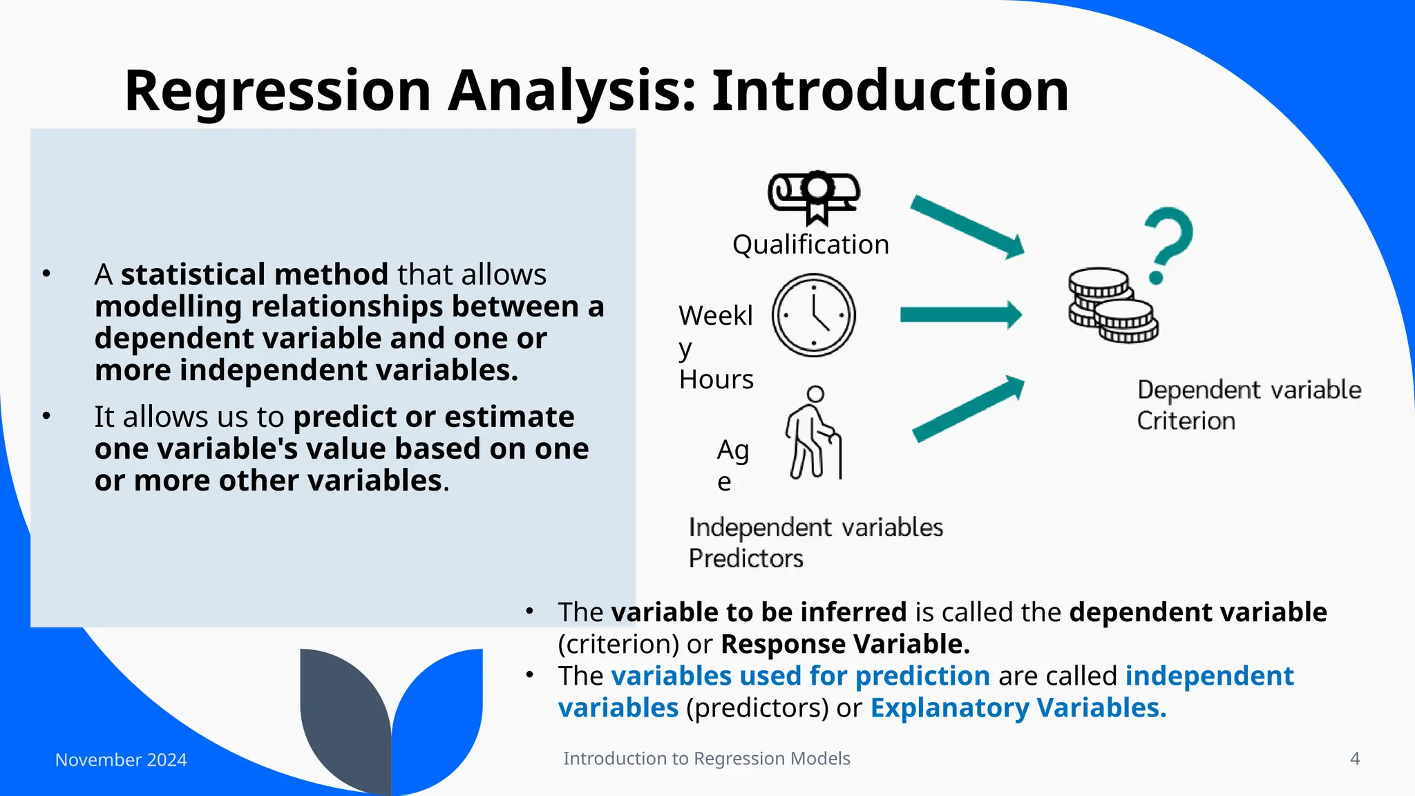
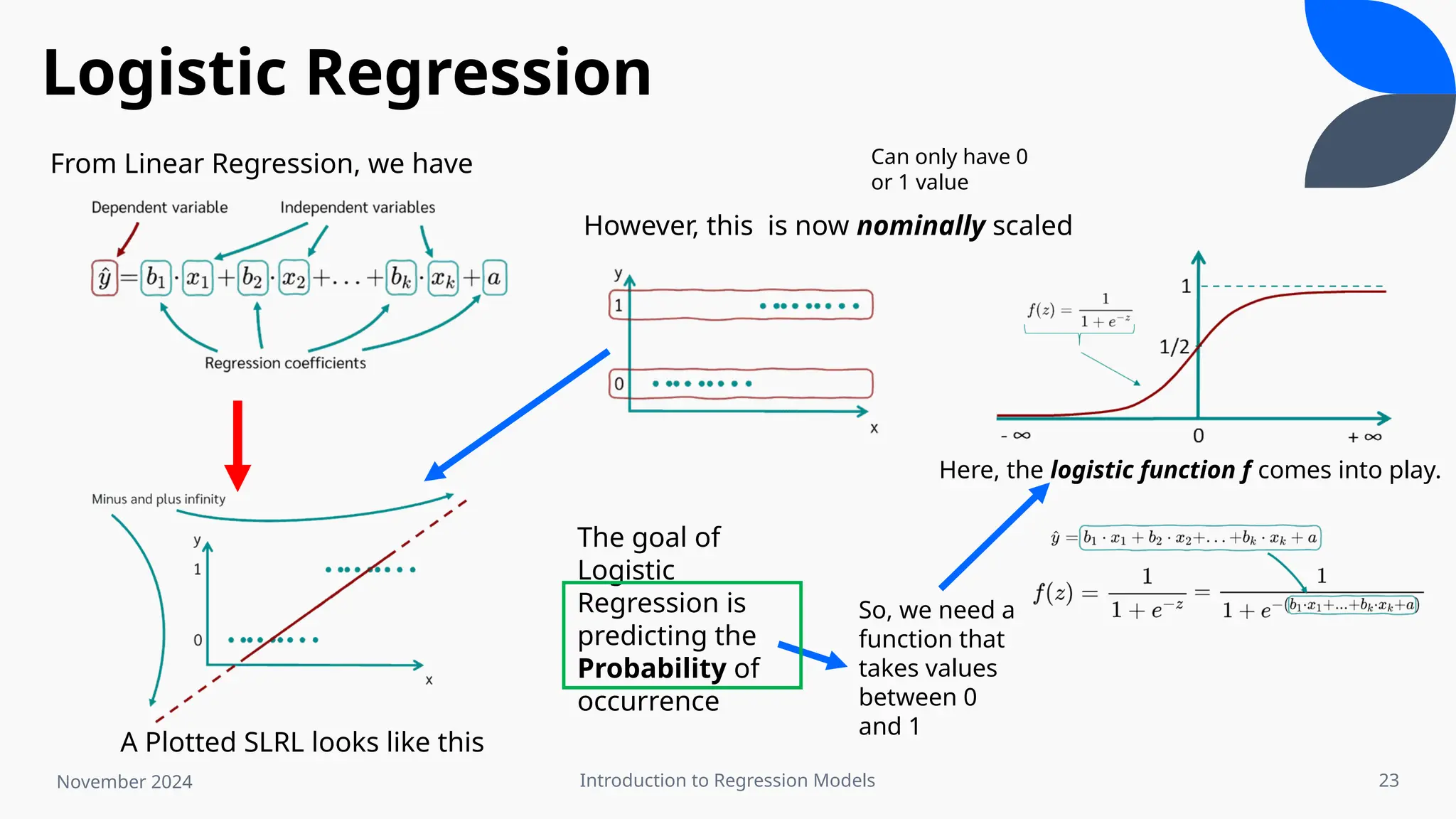
1. Regression
Models:
Multiple Linear &
Logistic
approaches

2. Introduction to Regression Models 2
Contents
Introduction to Regression Analysis.
Linear (Simple & Multiple) Regression Models.
Logistic Regression Model
References
November 2024

3. Introduction to Regression Models 3
An introduction to
Regression Analysis
November 2024

4. Introduction to Regression Models 4
Regression Analysis: Introduction
• A statistical method that allows
modelling relationships between a
dependent variable and one or
more independent variables.
• It allows us to predict or estimate
one variable's value based on one
or more other variables.
Qualification
Weekl
y
Hours
Ag
e
• The variable to be inferred is called the dependent variable
(criterion) or Response Variable.
• The variables used for prediction are called independent
variables (predictors) or Explanatory Variables.
November 2024

5. Introduction to Regression Models 5
Why is Regression
Analysis used?
It helps us examine
how one or more
variable might
influence another.
What factors affect
children's
concentration
abilities?
How do parents'
educational levels
and where they live
shape children’s
future educational
success?
It allows us to
forecast an
outcome based on
related variables.
How many days will
a patient likely stay
in the hospital?
What product is
someone most
inclined to buy
online?
November 2024

6. Introduction to Regression Models 6
Types of Regression Analysis
Choice of regression depends on the number of independent variables and the
measurement scale of the dependent variable.
Regression Type
No. of independent
variables
Scale of measurement of
Dependent Variable
Scale of Measurement
of Independent Variable
Simple Linear One Metric
Metric, Ordinal,
Nominal
Multiple Linear Multiple Metric
Metric, Ordinal,
Nominal
Logistic Multiple Ordinal, Nominal
Metric, Ordinal,
Nominal
November 2024

7. Introduction to Regression Models 7
Level of Measurement
Levels or Scales of measurement categorize variables based on how they're quantified.
Why are they important?
•Statistical Analysis: Different levels allow different statistical tests.
•Data Interpretation: Understanding the level helps interpret results accurately.
•Data Visualization: Appropriate visualization techniques depend on the level.
Level Characteristics Example
Nominal Categories only Gender, marital status
Ordinal Categories with order Education level, satisfaction rating
Interval
Numeric values with equal intervals, no true
zero
Temperature in Celsius or Fahrenheit
Ratio
Numeric values with equal intervals and a
true zero
Height, weight, income
November 2024

8. Introduction to Regression Models 8
Linear Regression
A specific type of regression analysis used when a clear, straight-line
relationship between the independent and dependent variables is
expected.
In mathematics, a linear relationship between two variables , is
given by,
• Visually, the relationship between 2
variables can be shown by a Scatter plot.
• Determine the straight line that best
describes the linear relationship in the
scatter plot, using method of Least
Squares.
• .
November 2024

9. Introduction to Regression Models 9
Types of Linear Regression
Simple Linear Regression:
• Involves 1 independent variable
(e.g., hours exercised) and 1
dependent variable (e.g., blood
pressure).
• Modelled using = +
𝑌 𝑎 𝑏𝑋, where 𝑎
is the intercept, 𝑏 is the slope, 𝑋 is
the independent variable, and 𝑌 is
the dependent variable.
• Goal: Find the best fit line to
predict based on
𝑌 𝑋.
Multiple Linear Regression:
• Involves multiple independent
variables (e.g., hours exercised, and
hours slept).
• Modelled using = +
𝑌 𝑎 , where and
represent slopes for each independent
variable with being the independent
variables.
• Goal: same as Simple linear regression;
to predict by considering multiple
𝑌
factors, making the model more
complex.
November 2024

10. Introduction to Regression Models 10
Regression Line:
• Shows how the response variable
(y) changes with the explanatory
variable (x), i.e., predict y for a
given x.
• Regression analysis identifies this
line and its direction of change,
using Sum of least squares method
• Represents the general trend,
though individual data points may
not align exactly with it.
November 2024
Related terminology:
𝒚 (Self Esteem) = (GPA) +
𝒎 ∙ 𝒙 C(intercept)
From this Graph,
• if GPA = 2.0, then self-esteem score = 78 or 79
(approx.)
• Intercept = 71 or 72 (approx.)
Now,
i.e., For Every point increase in GPA, Self-esteem score
increases by 4 points.

11. Introduction to Regression Models 11
Residuals:
• The difference between an observed value and its predicted value by the regression
line.
• Residuals indicate the error in prediction.
• Small residuals = Strong relationship (data points close to the line).Mean residual = 0.
• Residuals = +ve above the line & -ive below it.
November 2024
Related terminology:
Residuals are the deviations of
observed and predicted values

12. Introduction to Regression Models 12
Outliers & Influential Points:
• A data point far from others, often with a large residual is called an Outlier.
• An outlier in the x-direction that can significantly change the regression line, is called an
influential Point.
• Regression is sensitive to outliers, as coefficients rely on means, standard deviations, and
correlations.
• Removing outliers can improve the fit of the regression line and reduce residuals.
November 2024
Related Terminology:
• In graph (a), An Outlier exists with .
• In graph (b), Outlier Removed =
improves the regression line's fit by =
more accurate predictions.
(a) (b)
θ2
θ1
θ2> θ1

13. Introduction to Regression Models 13
Simple Linear Regression
• The most basic form with 1 independent
and 1 dependent variable.
• Determine the best values for 𝑎 and 𝑏 to
create the line of best fit.
• And then predict the dependent variable
based on the independent variable Weekly
Working
Hours
Hourly Salary
November 2024

14. Introduction to Regression Models 14
Simple Linear Regression
As we know, = +
𝑌 𝑎 𝑏𝑋
November 2024
a = 1.5 & b = 0.95
and,
1.5
Exp
(Yr)
Salary
(K$)

15. Introduction to Regression Models 15
R² or Coefficient of determination:
• Indicates the proportion of variance explained by independent variables.
Higher R² means a better model.
November 2024
Adjusted R²
Sum of squares of errors
Sum of squares of total
variance

16. Introduction to Regression Models 16
Assumptions of Linear Regression
To interpret the results of the regression analysis meaningfully, certain conditions
must be met.
• Linearity: There must be a linear relationship between the dependent and
independent variables.
• Homoscedasticity: The residuals must have a constant variance.
• Normality: Normally distributed error
• No multicollinearity: No high correlation between the independent variables
• No auto-correlation: The error component should have no auto correlation
November 2024

17. Introduction to Regression Models 17
Multiple Linear Regression
Extension of the simple linear regression model to two or
more independent variables
November 2024
Dependent
Variable Intercept/Bias
term Dependent
Variables
Coefficients of
Dependent variables
Intercept/Bias
term
Random Error

18. Introduction to Regression Models 18
Estimating Regression Parameters
For MLR, we observe rows of variables.
• Each row (or pair) is called a case, a
record, or a data point.
• is the response (or dependent
variable) of the observation
• There are p explanatory variables (or
covariates, predictors, independent
variables), and is the value of the
explanatory variable of the case
November 2024

19. Introduction to Regression Models 19
Estimating Regression Parameters
In SLR, Method of Least
Squares(LS) was used to
fit a line to the data. LS
estimates regression
parameters & .
For i= 1,2,..,n, can be
expressed equivalently
as
After A lot of
Calculations, we get;
Taking Derivate of this Q
function and setting it to
0 to find value of we get;
November 2024
Matrix Representation of
MLR

20. Introduction to Regression Models 20
Estimating Regression Parameters
Residuals( )
𝑒
The differences between the observed values and the predicted values:
R-Squared (Coefficient of Determination)
R-squared measures the proportion of the variance in the dependent variable that
is predictable from the independent variables:
Standard Error of the Estimate
The standard error of the estimate measures the standard deviation of the
residuals:
November 2024

21. Introduction to Regression Models 21
MLR : example dataset
November 2024
^
^
𝒀 (𝑺𝒄𝒐𝒓𝒆)=𝟏𝟎.𝟐𝟑+𝟎.𝟓𝟒(𝑯𝒐𝒖𝒓𝒔)+𝟎.𝟒𝟏( 𝑨𝒕𝒕𝒆𝒏𝒅𝒂𝒏𝒄𝒆)+𝟑.𝟐𝟓(𝑻𝒆𝒔𝒕𝒔)+𝝐

22. Introduction to Regression Models 22
Logistic Regression
• Used for binary (dichotomous)
dependent variables, predicting
outcomes like yes/no or 0/1.
• explains the relationship between a
binary dependent variable and one or
more independent variables.
• Linear regression predicts a dependent
variable's value, while logistic regression
estimates the probability of a
dichotomous outcome.
November 2024

23. Introduction to Regression Models 23
November 2024
Can only have 0
or 1 value
A Plotted SLRL looks like this
Here, the logistic function f comes into play.
From Linear Regression, we have
However, this is now nominally scaled
The goal of
Logistic
Regression is
predicting the
Probability of
occurrence
So, we need a
function that
takes values
between 0
and 1
Logistic Regression

24. Introduction to Regression Models 24
November 2024
Log-Likelihood (LL):
Measures how well the model fits:
A higher indicates better fit.
𝐿𝐿
Maximum Likelihood Estimation (MLE)
finds optimal _0​and _1​(for which
𝒃 𝒃
LL is as close to zero as possible).
Unlike linear regression (which uses Ordinary Least Squares), Maximum Likelihood
Estimation (MLE) is used for parameter estimation in logistic regression.
There are infinite possible sets of regression coefficients, and MLE finds the set
that maximizes the probability of observing the given data.
Estimation of Regression
Coefficients

25. Thank you

26. References:
November 2024 Introduction to Regression Models 26
• https://datatab.net/tutorial/regression
• https://www.javatpoint.com/regression-analysis-in-m
achine-learning
• https://www.youtube.com/@statquest
• Darlington, R. B., & Hayes, A. F. (2017). Regression
analysis and linear models: Concepts, applications,
and implementation. Guilford Press.
• Anderson, A. Business Statistics For Dummies®.
Wiley, 2015.
• Graybill, F. A., & Iyer, H. K. (2017). Regression analysis:
Concepts and applications. Duxbury Press.