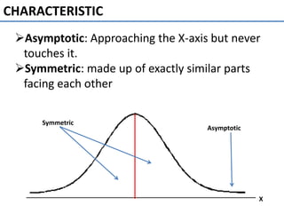
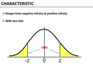
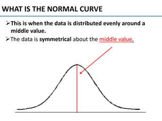
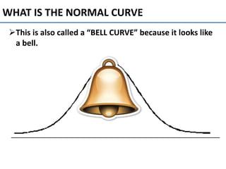
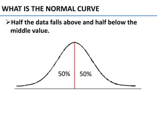
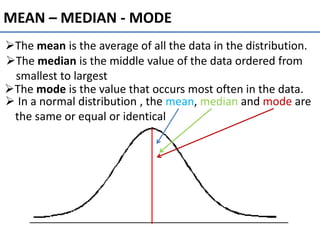
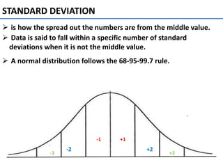
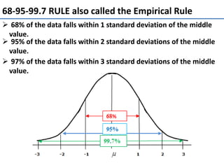
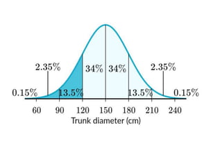
2. HISTORY
Began in the middle of 18th
century with the work of
Abraham DeMoivre
Marquis de
Laplace
At the beginning of 19th century
Karl Friedrich made substantial
contributions. And scientist called it
the “Laplace-Gaussian Curve”.
Karl Pearson is credited with
being first to refer to the
curve as the “Normal curve
3. IMPORTANCE
One reason the normal distribution is important
is that many psychological and educational
variables are distributed approximately
normally.
-Measures of reading ability,
introversion, job satisfaction, and memory
are among the many psychological variables
approximately normally distributed.
-Although the distributions are only
approximately normal, they are usually
quite close.
4. IMPORTANCE
The second reason the normal distribution is so
important is that it is easy for mathematical statisticians
to work with.
-This means that many kinds of statistical tests can
be derived for normal distributions.
-Almost all statistical tests discussed in this text
assume normal distributions.
-Fortunately, these tests work very well even if the
distribution is only approximately normally
distributed.
-Some tests work well even with very wide
deviations from normality.
7. WHAT IS THE NORMAL CURVE
This is when the data is distributed evenly around a
middle value.
The data is symmetrical about the middle value.
8. WHAT IS THE NORMAL CURVE
This is also called a “BELL CURVE” because it looks like
a bell.
9. WHAT IS THE NORMAL CURVE
Half the data falls above and half below the
middle value.
50% 50%
10. MEAN – MEDIAN - MODE
The mean is the average of all the data in the distribution.
The median is the middle value of the data ordered from
smallest to largest
The mode is the value that occurs most often in the data.
In a normal distribution , the mean, median and mode are
the same or equal or identical
11. STANDARD DEVIATION
is how the spread out the numbers are from the middle value.
Data is said to fall within a specific number of standard
deviations when it is not the middle value.
-1 +1
-2 +2
-3 +3
A normal distribution follows the 68-95-99.7 rule.
12. 68-95-99.7 RULE also called the Empirical Rule
68% of the data falls within 1 standard deviation of the middle
value.
95% of the data falls within 2 standard deviations of the middle
value.
97% of the data falls within 3 standard deviations of the middle
value.
13. PERCENT AT EACH STANDARD DEVIATION
The middle value represents 50%.
Recall that 68% of the data falls within 1 standard
deviation of the mean.
Half the 68% falls above and half below 50%.
1 standard deviation below the mean is 50% - 34% = 16%
1 standard deviation above the mean is 50% + 34% = 84%
14. PERCENT AT EACH STANDARD DEVIATION
Recall that 95% of the data falls within 2 standard
deviations of the mean.
Half the 95% falls above and half below 50%.
2 standard deviations below the mean is 50% - 47.5% = 2.5%
2 standard deviations above the mean is 50% + 47.5% = 97.5%
15. PERCENT AT EACH STANDARD DEVIATION
Recall that 99.7% of the data falls within 3 standard
deviations of the mean.
Half the 99.7% falls above and half below 50%.
3standard deviations below the mean is 50% - 49.85% = .15%
3 standard deviations above the mean is 50% + 49.85% = 99.85%
16. HOW TO USE NORMAL CURVE TO DETERMINE
PROBABILITY
Determine the mean. (µ)
Determine the standard deviation. (ơ)
Plot the mean and SD on the
normal curve.
Analyze the problem.
Apply the 68-95-99.7 or empirical rule
17. Practice
The normal distribution below has a standard deviation of 10.
Approximately what area contained between 70 and 90?
40 60 70 80 90 10050
Mean= 70
SD= 10
18. Practice
For the normal distribution below, approximately what area
contained between -2 and 1
1-1 2 30-3 -2
Mean = 0
SD= 1
19. Practice
A certain variety of pine tree has a mean trunk
diameter of µ=150cm and a standard deviation of
ơ=30cm.
A certain section of a forest has 500 of these
trees.
Approximately how many of these trees have
a diameter of between 120 and 180
centimeters?