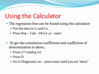
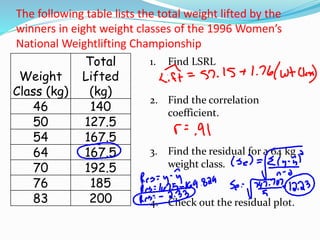
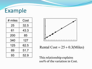
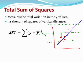
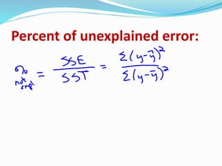
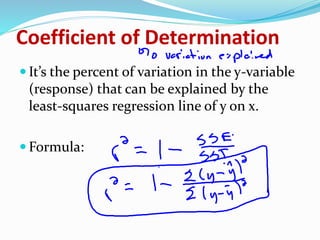
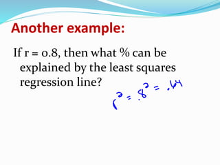
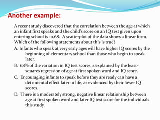
The document provides information about regression analysis and calculating the coefficient of determination. It includes: 1) Instructions on how to perform a regression analysis using a calculator to find the least squares regression line, correlation coefficient, and residual plot from sample data. 2) An explanation of the coefficient of determination as a measure of how much variability in the variable y can be explained by its linear relationship with variable x. 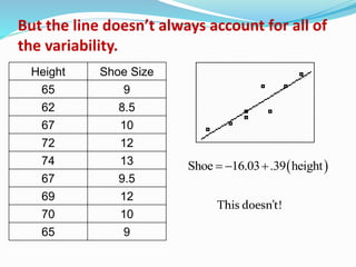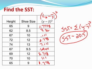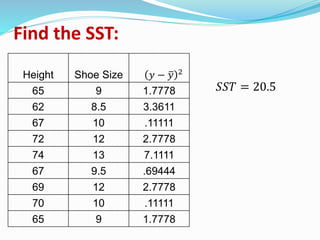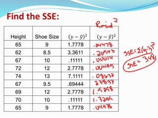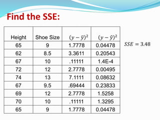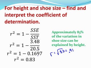3) A calculation example finding the coefficient of determination to be 0.83 for a dataset relating height and shoe size, meaning approximately 83% of the variation in shoe size can be explained by height.

1. Section 3.2C

2.  The regression line can be found using the calculator
 Put the data in L1 and L2.
 Press Stat – Calc - #8 (or 4) - enter
 To get the correlation coefficient and coefficient of
determination to show…
 Press 2nd catalog (0)
 Press D
 Go to Diagnostic on – press enter until you see “done”
Using the Calculator

3. The following table lists the total weight lifted by the
winners in eight weight classes of the 1996 Women’s
National Weightlifting Championship
Weight
Class (kg)
Total
Lifted
(kg)
46 140
50 127.5
54 167.5
64 167.5
70 192.5
76 185
83 200
1. Find LSRL
2. Find the correlation
coefficient.
3. Find the residual for a 64 kg
weight class.
4. Check out the residual plot.

4. If a line is appropriate, then we
need to assess the accuracy of
predictions based on the least
squares line.

5. Coefficient of Determination
It’s the measure of the proportion of
variability in the variable that can be
“explained” by a linear relationship
between the variables x and y.

6. Example
# miles Cost
25 32.5
61 43.3
200 85
340 127
125 62.5
89 51.7
93 52.9
Rental Cost 25 0.3(Miles) 
This relationship explains
100% of the variation in Cost.

7. But the line doesn’t always account for all of
the variability.
Height Shoe Size
65 9
62 8.5
67 10
72 12
74 13
67 9.5
69 12
70 10
65 9
 Shoe 16.03 .39 height  
This doesn’t!

8. Total Sum of Squares
 Measures the total variation in the y-values.
 It’s the sum of squares of vertical distances
𝑺𝑺𝑻 = 𝒚 − 𝒚 𝟐

9. Find the SST:
Height Shoe Size 𝑦 − 𝑦 2
65 9
62 8.5
67 10
72 12
74 13
67 9.5
69 12
70 10
65 9

10. Find the SST:
Height Shoe Size 𝑦 − 𝑦 2
65 9 1.7778
62 8.5 3.3611
67 10 .11111
72 12 2.7778
74 13 7.1111
67 9.5 .69444
69 12 2.7778
70 10 .11111
65 9 1.7778
𝑆𝑆𝑇 = 20.5

11. Sum of Squared Errors
This is the sum of the squared residuals
Total of the unexplained error
Formula: 𝑆𝑆𝐸 = 𝑦 − 𝑦 2

12. Find the SSE:
Height Shoe Size 𝑦 − 𝑦 2 𝑦 − 𝑦 2
65 9 1.7778
62 8.5 3.3611
67 10 .11111
72 12 2.7778
74 13 7.1111
67 9.5 .69444
69 12 2.7778
70 10 .11111
65 9 1.7778

13. Find the SSE:
Height Shoe Size 𝑦 − 𝑦 2 𝑦 − 𝑦 2
65 9 1.7778 0.04478
62 8.5 3.3611 0.20543
67 10 .11111 1.4E-4
72 12 2.7778 0.00495
74 13 7.1111 0.08632
67 9.5 .69444 0.23833
69 12 2.7778 1.5258
70 10 .11111 1.3295
65 9 1.7778 0.04478
𝑆𝑆𝐸 = 3.48

14. Percent of unexplained error:

15. Coefficient of Determination
 It’s the percent of variation in the y-variable
(response) that can be explained by the
least-squares regression line of y on x.
 Formula:

16. For height and shoe size – find and
interpret the coefficient of
determination.
𝑟2
= 1 −
𝑆𝑆𝐸
𝑆𝑆𝑇

17. For height and shoe size – find and
interpret the coefficient of
determination.
𝑟2
= 1 −
𝑆𝑆𝐸
𝑆𝑆𝑇
𝑟2
= 1 −
3.48
20.5
𝑟2
= 1 − 0.1697
𝑟2
= 0.83
Approximately 83%
of the variation in
shoe size can be
explained by height.

18. Find the Coefficient of Determination:
Team Batting
Avg.
Mean # runs
per
game
0.289 5.9
0.279 5.5
0.277 4.9
0.274 5.2
0.271 4.9
0.271 5.4
0.268 4.5
0.268 4.6
0.266 5.1

19. Interpret this in context…
59.5% of the observed variability in
mean number of runs per game can be
explained by an approximate linear
relationship between Team Batting
average and mean runs per game.

20. Another example:
If r = 0.8, then what % can be
explained by the least squares
regression line?

21. Another example:
A recent study discovered that the correlation between the age at which
an infant first speaks and the child’s score on an IQ test given upon
entering school is -0.68. A scatterplot of the data shows a linear form.
Which of the following statements about this is true?
A. Infants who speak at very early ages will have higher IQ scores by the
beginning of elementary school than those who begin to speak
later.
B. 68% of the variation in IQ test scores is explained by the least-
squares regression of age at first spoken word and IQ score.
C. Encouraging infants to speak before they are ready can have a
detrimental effect later in life, as evidenced by their lower IQ
scores.
D. There is a moderately strong, negative linear relationship between
age at first spoken word and later IQ test score for the individuals
this study.

22. Homework
 Page 192 (49, 51, 54, 56, 58, 71-78)