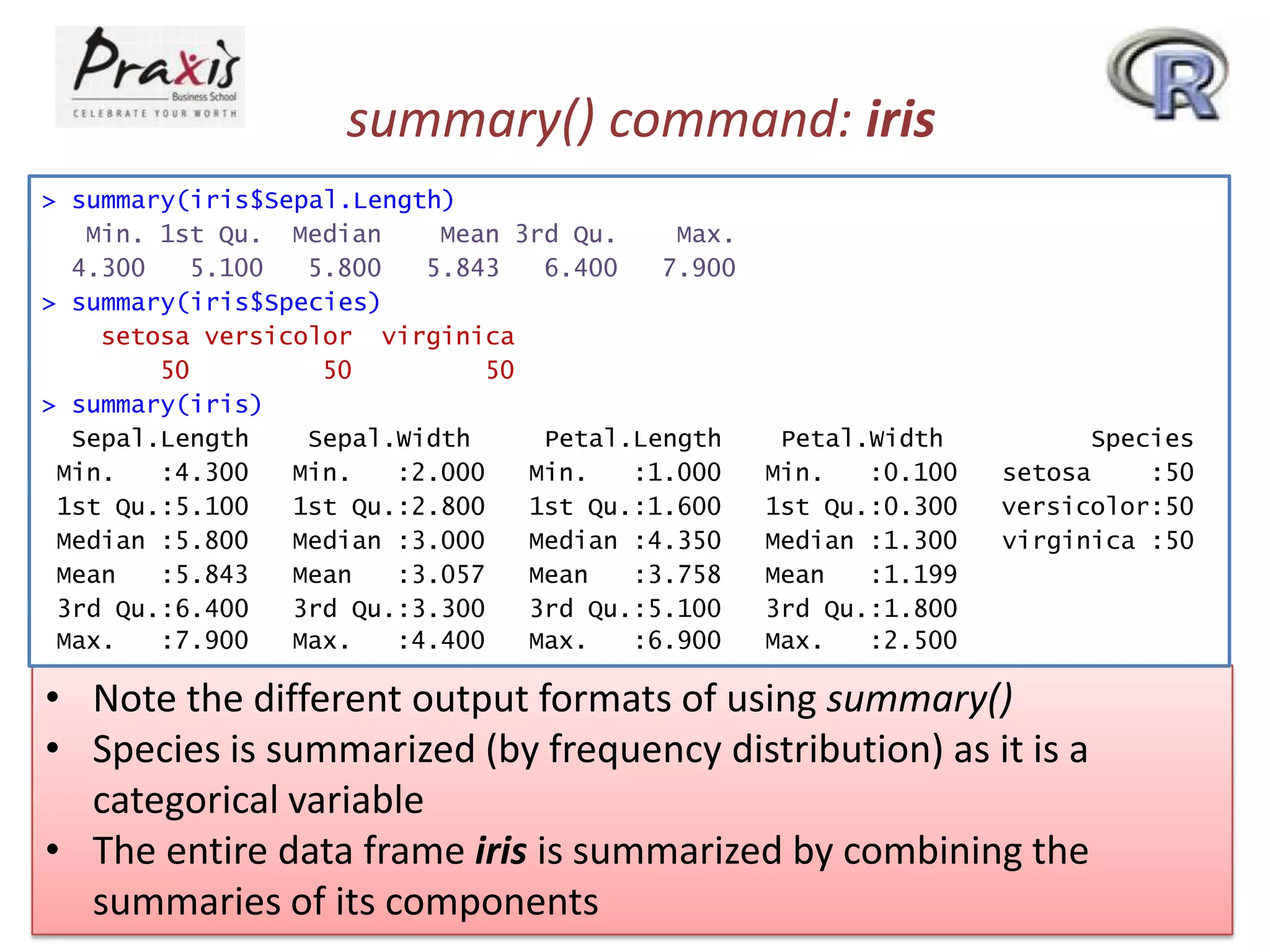
- The document demonstrates various commands for exploring and summarizing data in R such as the iris data set including head(), tail(), str(), class(), summary(), and $-operator. - The iris data set contains measurement data for 150 flowers across 4 variables and is stored as a data frame object in R. - Data frames allow storing different data types together and can be explored using commands like summary() which provides summaries tailored to each variable type. - Matrices can also be used to store multi-dimensional data and various functions like dim(), apply(), and cbind() allow manipulating the dimensions and combining matrices.

1. Data available in R
> data()
> data("AirPassengers")
> head(AirPassengers)
[1] 112 118 132 129 121 135
> tail(AirPassengers)
[1] 622 606 508 461 390 432
> str(AirPassengers)
Time-Series [1:144] from 1949 to 1961: 112 118 132 129 121 135 148 148
136 119 ...
> class(AirPassengers)
[1] "ts"
> help(ts)
• The command data() loads data-sets available in R
• head() and tail() command displays first few or last few
values
• str() shows the structure of an R object
• class() shows the class of an R object
• What does “ts” stand for?

2. Try runif() and plot() commands ….
runif(10)
[1] 0.14350413 0.54293576 0.62881627 0.30278850 0.28030129 0.03784996
0.49483957
[8] 0.23571517 0.40072956 0.20327478
> plot(runif(10))
The runif()
command generates
U(0,1)10 random
numbers between 0
and 1.
These numbers have
been plotted by the
plot() function.

3. A dataset in R: iris
> head(iris)
Sepal.Length Sepal.Width Petal.Length Petal.Width Species
1
5.1
3.5
1.4
0.2 setosa
2
4.9
3.0
1.4
0.2 setosa
3
4.7
3.2
1.3
0.2 setosa
4
4.6
3.1
1.5
0.2 setosa
5
5.0
3.6
1.4
0.2 setosa
6
5.4
3.9
1.7
0.4 setosa
> tail(iris)
Sepal.Length Sepal.Width Petal.Length Petal.Width
145
6.7
3.3
5.7
2.5
146
6.7
3.0
5.2
2.3
147
6.3
2.5
5.0
1.9
148
6.5
3.0
5.2
2.0
149
6.2
3.4
5.4
2.3
150
5.9
3.0
5.1
1.8
Species
virginica
virginica
virginica
virginica
virginica
virginica
The iris dataset contains measurement of 150 flowers, 50
each from 3 species : iris setosa, versicolor and virginica.

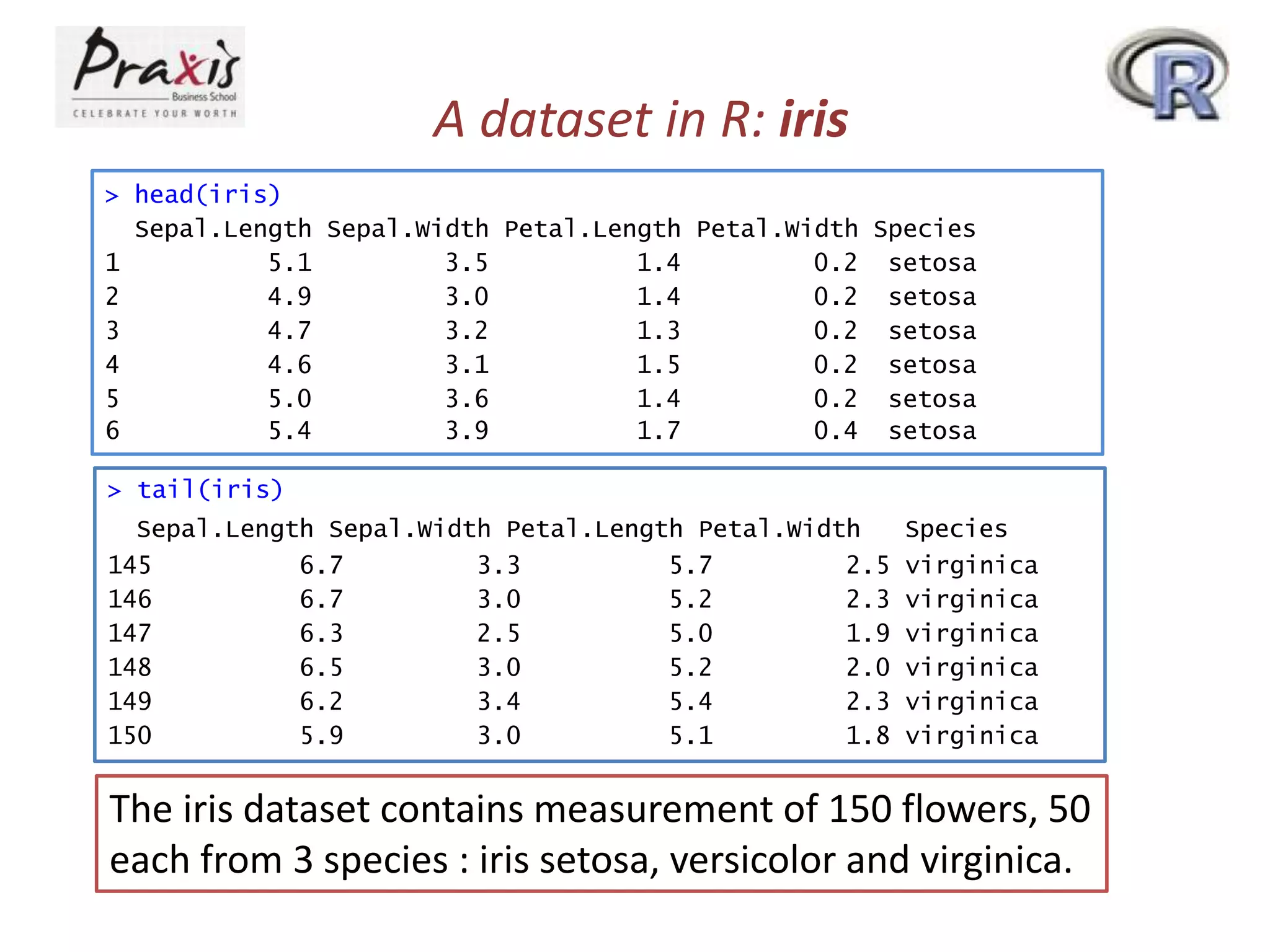
4. Data frame in R: iris
> str(iris)
'data.frame':
150 obs. of 5 variables:
$ Sepal.Length: num 5.1 4.9 4.7 4.6 5 5.4 4.6 5 4.4 4.9 ...
$ Sepal.Width : num 3.5 3 3.2 3.1 3.6 3.9 3.4 3.4 2.9 3.1 ...
$ Petal.Length: num 1.4 1.4 1.3 1.5 1.4 1.7 1.4 1.5 1.4 1.5 ...
$ Petal.Width : num 0.2 0.2 0.2 0.2 0.2 0.4 0.3 0.2 0.2 0.1 ...
$ Species
: Factor w/ 3 levels "setosa","versicolor",..: 1 1 1 1 1
1 1 1 1 1 ...
> class(iris)
[1] "data.frame"
• As you see, iris is not a simple vector but a composite
“data frame” object made up of several component
vectors as you can see in the output of class(iris)
• You can think of a data frame as a matrix-like object
- each row for each observational unit (here, a flower)
- each column for each measurement made on the unit
• But the str() function gives you more concise description
on iris.

5. Use of $ operator: iris
> iris$Sepal.Length
[1] 5.1 4.9 4.7 4.6
5.7 5.1
[21] 5.4 5.1 4.6 5.1
4.4 5.1
[41] 5.0 4.5 4.4 5.0
6.6 5.2
[61] 5.0 5.9 6.0 6.1
6.0 5.7
[81] 5.5 5.5 5.8 6.0
5.1 5.7
[101] 6.3 5.8 7.1 6.3
7.7 6.0
[121] 6.9 5.6 7.7 6.3
6.0 6.9
[141] 6.7 6.9 5.8 6.8
5.0 5.4 4.6 5.0 4.4 4.9 5.4 4.8 4.8 4.3 5.8 5.7 5.4 5.1
4.8 5.0 5.0 5.2 5.2 4.7 4.8 5.4 5.2 5.5 4.9 5.0 5.5 4.9
5.1 4.8 5.1 4.6 5.3 5.0 7.0 6.4 6.9 5.5 6.5 5.7 6.3 4.9
5.6 6.7 5.6 5.8 6.2 5.6 5.9 6.1 6.3 6.1 6.4 6.6 6.8 6.7
5.4 6.0 6.7 6.3 5.6 5.5 5.5 6.1 5.8 5.0 5.6 5.7 5.7 6.2
6.5 7.6 4.9 7.3 6.7 7.2 6.5 6.4 6.8 5.7 5.8 6.4 6.5 7.7
6.7 7.2 6.2 6.1 6.4 7.2 7.4 7.9 6.4 6.3 6.1 7.7 6.3 6.4
6.7 6.7 6.3 6.5 6.2 5.9
Note that $-operator extracts individual components of a data
frame.
Try summary() and IQR() commands on iris$Sepal.Length
and study the data

6. summary() command: iris
> summary(iris$Sepal.Length)
Min. 1st Qu. Median
Mean 3rd Qu.
Max.
4.300
5.100
5.800
5.843
6.400
7.900
> summary(iris$Species)
setosa versicolor virginica
50
50
50
> summary(iris)
Sepal.Length
Sepal.Width
Petal.Length
Min.
:4.300
Min.
:2.000
Min.
:1.000
1st Qu.:5.100
1st Qu.:2.800
1st Qu.:1.600
Median :5.800
Median :3.000
Median :4.350
Mean
:5.843
Mean
:3.057
Mean
:3.758
3rd Qu.:6.400
3rd Qu.:3.300
3rd Qu.:5.100
Max.
:7.900
Max.
:4.400
Max.
:6.900
Petal.Width
Min.
:0.100
1st Qu.:0.300
Median :1.300
Mean
:1.199
3rd Qu.:1.800
Max.
:2.500
Species
setosa
:50
versicolor:50
virginica :50
• Note the different output formats of using summary()
• Species is summarized (by frequency distribution) as it is a
categorical variable
• The entire data frame iris is summarized by combining the
summaries of its components

7. class() command: iris
> class(iris$Sepal.Length)
[1] "numeric"
> class(iris$Species)
[1] "factor"
> class(iris)
[1] "data.frame"
• Note that each R object has a class (“numeric”, “factor” etc.)
• summary() is referred to as a generic function
• When summary() is applied, R figures out the appropriate
method and calls it

8. More on summary() command
> methods(summary)
[1] summary.aov
[4] summary.connection
[7] summary.default
[10] summary.glm
[13] summary.loess*
[16] summary.mlm
[19] summary.PDF_Dictionary*
[22] summary.POSIXlt
[25] summary.princomp*
[28] summary.stepfun
[31] summary.tukeysmooth*
summary.aovlist
summary.data.frame
summary.ecdf*
summary.infl
summary.manova
summary.nls*
summary.PDF_Stream*
summary.ppr*
summary.srcfile
summary.stl*
summary.aspell*
summary.Date
summary.factor
summary.lm
summary.matrix
summary.packageStatus*
summary.POSIXct
summary.prcomp*
summary.srcref
summary.table
Non-visible functions are asterisked
• Objects of class “factor” are handled by summary.factor()
• “data.frame”s are handled by summary.data.frame()
• Numeric vectors are handled by summary.default()

9. Try the following ….
•
•
•
•
•
•
•
•
•
attach() and detach() with iris
xx <- 1:12 and then dim(xx) <- c(3,4)
apply nrow(xx) and ncol(xx)
dim(xx) <- c(2,2,3)
yy <- matrix(1:12, nrows=3, byrow=TRUE
rownames(yy) <- LETTERS[1:3]
use colnames()
zz <- cbind(A=1:4, B=5:8, C=9:12)
rbind(zz,0)