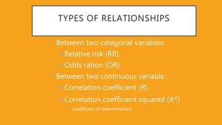
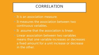
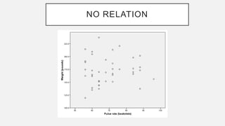
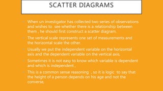
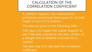
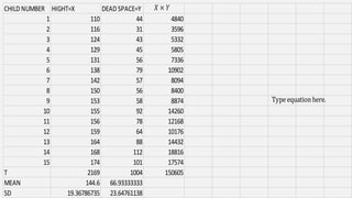
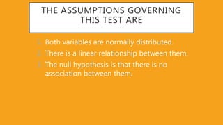
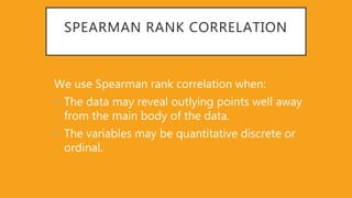
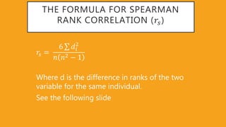
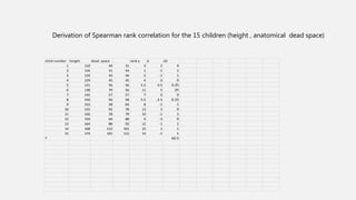
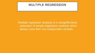
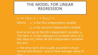
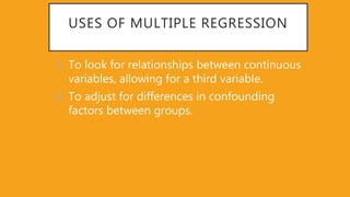
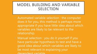
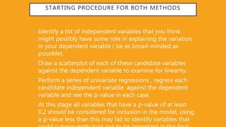
SlideShare a Scribd company logo
CORRELATION AND REGRESSION
Dr Abdul Aziz Tayoun
Consultant community medicine
Supervisor training center –SBPM
(Rawdhah)
TYPES OF RELATIONSHIPS
• Between two categorial variables:
Relative risk (RR).
Odds ration (OR).
• Between two continuous variable :
Correlation coefficient (R).
Correlation coefficient squared (𝑅2
)
(coefficient of determination)
CORRELATION
 It is an association measure.
 It measures the association between two
continuous variables.
 It assume that the association is linear.
 Linear association between two variables
means that one variable increases or decreases
a fixed amount for a unit increase or decrease
in the other.
CORRELATION COEFFICIENT
• It measures the degree of association .
• It measures linear association.
• It is sometimes called Pearson’s correlation
coefficient.
STRENGTH OF ASSOCIATION
• The correlation coefficient is measured on a
scale that varies from +1 through 0 to -1.
• Complete correlation between two variables is
expressed by either +1 or -1.
• When one variable increases as the other
increases the correlation is positive.
• When one decreases as the other increases it
is negative.
• Complete absence of correlation is
represented by 0.
POSITIVE RELATIONSHIP
NEGATIVE RELATIONSHIP
Reliability
Age of Car
NO RELATION
SCATTER DIAGRAMS
• When un investigator has collected two series of observations
and wishes to see whether there is a relationship between
them , he should first construct a scatter diagram.
• The vertical scale represents one set of measurements and
the horizontal scale the other.
• Usually we put the independent variable on the horizontal
axis and the dependent variable on the vertical axis,
• Sometimes it is not easy to know which variable is dependent
and which is independent ,
• This is a common sense reasoning , so it is logic to say that
the height of a person depends on his age and not the
converse,
CALCULATION OF THE
CORRELATION COEFFICIENT
• A pediatric registrar has measured the
pulmonary anatomical dead space (in ml) and
height in (cm) of 15 children.
• The data are given in the following table.
• First step is to inspect the scatter diagram to
see if the area covered by the dots centers on
a straight line or whether a curved line is
needed.
• The next step is to calculate the correlation
coefficient
CHILD NUMBER HIGHT=X DEAD SPACE=Y
1 110 44 4840
2 116 31 3596
3 124 43 5332
4 129 45 5805
5 131 56 7336
6 138 79 10902
7 142 57 8094
8 150 56 8400
9 153 58 8874
10 155 92 14260
11 156 78 12168
12 159 64 10176
13 164 88 14432
14 168 112 18816
15 174 101 17574
T 2169 1004 150605
MEAN 144.6 66.93333333
SD 19.36786735 23.64761138
HIGHT=X DEAD SPACE=Y
110 44
116 31
124 43
129 45
131 56
138 79
142 57
150 56
153 58
155 92
156 78
159 64
164 88
168 112
174 101
0
20
40
60
80
100
120
0 50 100 150 200
deadspace hieghte
scatter graph of height and anatomic dead space
for the 15 children
THE FORMULA TO BE USED
With x representing the value of independent variable(in this
case the height) and y representing the dependent variable ( in
this case the anatomical dead space):
𝑟 =
𝑥 − 𝑥 𝑦 − 𝑦
𝑥 − 𝑥 2 (𝑦 − 𝑦)2
Which can be shown to be equal to :
𝑟 =
𝑥𝑦 − 𝑛 𝑥 𝑦
𝑛 − 1 𝑆 𝑥 𝑆 𝑦
Where : x = height in cm
y = anatomical dead space in ml
𝑥 = mean of height 𝑦 = mean of anatomical dead
space
𝑆 𝑥= standard deviation for height 𝑆 𝑦= standard
deviation for anatomical dead space
CALCULATION
𝑟 =
150605 − 15 144 6 66 93
14 19 37 23 65
𝑟 =
150605 − 145171 17
5412 06
=
5433,83
6412,0609
= 0 847
𝑅2
= 0 8472
= 0,717
COMMENTS ON THE RESULTS
• The correlation coefficient of 0.817 indicates a positive
correlation between the size of the pulmonary anatomical
dead space and height of the child .
• But in the interpretation of correlation it is important to
remember that correlation is not causation.
• A part of the variation in one of the variables (as measured by
it’s variance) can be thought of as being due to the
relationship with the other variable and another part as due
to undetermined often random causes.
• The part due to the dependence of one variable on the other
can be measured by 𝑅2 and it is equal to 0.717 in our
example.
• So we can say that 72% of the variation between children in
the size of anatomical dead space is due to the height of the
child.
•
The value of r ranges between ( -1) and ( +1)
The value of r denotes the strength of the
association as illustrated
by the following diagram.
-1 10-0.25-0.75 0.750.25
strong strongintermediate intermediateweak weak
no relation
perfect
correlation
perfect
correlation
Directindirect
SIGNIFICANCE TEST FOR
CORRELATION COEFFICIENT
To test wether the association is merely
apparent , and might have been arisen by
chance , we use the ( t test) with the following
equation :
𝑡 = 𝑟
𝑛 − 2
1 − 𝑟2
We must enter the t table with n-2 degrees of
freedom
CALCULATION OF T
𝑡 = 0 847
15−2
1−0 8472 = 0 847
13
0 283
= 0.847 45 9
=5.74
If we enter the t table with (15-2=13) degrees
of freedom
We find p < 0.001
So the correlation coefficient may be regarded
as highly significant .
Thus we have a very strong correlation between
dead space and height of the child , which is
most unlikely have arisen by chance.
THE ASSUMPTIONS GOVERNING
THIS TEST ARE
1. Both variables are normally distributed.
2. There is a linear relationship between them.
3. The null hypothesis is that there is no
association between them.
SPEARMAN RANK CORRELATION
We use Spearman rank correlation when:
• The data may reveal outlying points well away
from the main body of the data.
• The variables may be quantitative discrete or
ordinal.
THE FORMULA FOR SPEARMAN
RANK CORRELATION (𝑟𝑠)
𝑟𝑠 =
6 𝑑𝑖
2
𝑛 𝑛2 − 1
Where d is the difference in ranks of the two
variable for the same individual.
See the following slide
child number height dead space rank y d d2
1 110 44 31 3 2 4
2 116 31 43 1 -1 1
3 124 43 44 2 -1 1
4 129 45 45 4 0 0
5 131 56 56 5.5 0.5 0.25
6 138 79 56 11 5 25
7 142 57 57 7 0 0
8 150 56 58 5.5 -2.5 6.25
9 153 58 64 8 -1 1
10 155 92 78 13 3 9
11 156 78 79 10 -1 1
12 159 64 88 9 -3 9
13 164 88 92 12 -1 1
14 168 112 101 15 1 1
15 174 101 112 14 -1 1
T 60.5
Derivation of Spearman rank correlation for the 15 children (height , anatomical dead space)
CALCULATION OF SPEARMAN
RANK CORRELATION
𝑟𝑠 = 1 −
6 60 5
15 225−1
= 1 −
383
15 224
= 1 −
363
3360
= 1 −
0 108 = 0 892
In this case the value is very close to the Pearson
correlation coefficient .
For more than n >10 , the Spearman rank
correlation can be tested for significance using
the t test.
LINEAR REGRESSION
DIFFERENCE BETWEEN CORRELATION
AND REGRESSION
• Correlation describes the strength of
association between two variables and
completely symmetrical , the correlation
between A & B is the same as the correlation
between B & A , if one variable change by a
certain amount the other changes on average
by a certain amount.
• The regression equation representing how
much the dependent variable changes with
any given change in the independent
variables, which can be used to construct a
REGRESSION
Calculates the “best-fit” line for a certain set of data
The regression line makes the sum of the squares of
the residuals smaller than for any other line
Regression minimizes residuals
80
100
120
140
160
180
200
220
60 70 80 90 100 110 120
Wt (kg)
SBP(mmHg)
ASSUMPTIONS FOR THE ORDINARY
LEAST SQUARES PROCEDURE
1. The relationship between X and Y is linear.
2. The dependent variable Y is metric
continuous
3. The residual term e , is normally distributed,
with a mean of zero , for each value of the
independent variable X.
4. The spread of the residual terms should be
the same, whatever the value of X.
HOW TO CALCULATE b
HOW TO CALCULATE a
REGRESSION EQUATION
Regression equation
describes the
regression line
mathematically
• Intercept
• Slope
80
100
120
140
160
180
200
220
60 70 80 90 100 110 120
Wt (kg)
SBP(mmHg)
LINEAR EQUATIONS
Y
Y = bX + a
a = Y-intercept
X
Change
in Y
Change in X
b = Slope
INTERPRETATION OF THE
EQUATION
X : represents the independent variable
Y : represents the dependent variable.
a : represents the intercept , the value of y when x=0
b : represents the slope , the value of y when x
changes by one unit.
So the regression equation is more useful than the
correlation coefficient because it allows us to predict
the value of y when we know the value of x.
CALCULATION OF THE REGRESSION
MODEL
𝑏 =
𝑥 𝑦 −𝑛 𝑥 𝑦
𝑛−1 𝑆 𝑥
2
𝑎 = 𝑦- b 𝑥
𝑏 =
150605−15 144 6 66 93
14 19 36972 =
5433 83
5251 6
= 1.033
𝑎 = 66 93 − 1 033 144 6 = 66 93 − 149 37
= −82.4
Y= -82.4 + 1.033 x
INTERPRETATION OF THE RESULTS
• when the height is 0 the anatomical dead
space is – 82.4 which is not logic, the
equitation is valid only for the range between
minimum and maximal height regarding the
data , say between 110- 174 cm only.
• For every centimeter increase in the height the
anatomical dead space increases by 1.033 ml
over the range of measurement mode.
TESTING THE HYPOTHESIS B=0
𝑡 =
𝑏
𝑆𝐸(𝑏)
SE(b)=
𝑆 𝑟𝑒𝑠
𝑥− 𝑥 2
=
𝑆 𝑟𝑒𝑠
𝑛−1 𝑆 𝑥
2
𝑆𝑟𝑒𝑠=
𝑦−𝑦 𝑓𝑖𝑡
2
𝑛−2
This can be shown algebraically equal to :
𝑆𝑟𝑒𝑠 =
𝑆 𝑦
2
1 − 𝑟2 𝑛 − 1
𝑛 − 2
CALCULATION OF STANDARD ERROR
OF B
𝑆𝑟𝑒𝑠 =
23 652 1−0 8462 15−1
15−2
=
559 133 0,284 14
13
=
2225 36
13
= 171 18 =13.08
𝑆𝐸 𝑏 =
𝑆 𝑟𝑒𝑠
𝑛−1 𝑆 𝑥
2
=
13 08
14 19 36792
=
13 08
5251 6
=
13 08
72,468
= 0.1805
𝑡 =
1 033
0 1805
= 5.72
This has 15-2 =13 degrees of freedom
p value < 0.001
Note that the test significance for the slope gives exactly the
same value of p as the test of significance for the correlation
coefficient., although the two tests are derived differently.
95% CONFIDENCE INTERVAL FOR B
95% CI forb = 𝑏 ± 𝑡0 05 𝑆𝐸(𝑏)
95% 𝐶𝐼 𝑓𝑜𝑟 𝑏 = 1 033 ± 2 16 0 1805
= 1 033 ± 0 3899
95%CI for b = (0.643 to 1.423)
FROM THE REGRESSION MODEL WE
CAN CALCULATE THE VALUE OF Y FOR
ANY VALUE OF X
Question : what is the anatomical dead space
for a child measuring 125 and 150 cm?
Answer : 𝑦 = −82 4 + 1 033 𝑥
Y = -82.4 +1.033 *125 =46,725 ml
Y= -82.4+ 1.033*150 = 72.55 mi
THE ASSUMPTIONS ARE
1. The prediction error are approximately
Normally distributed, note that this does not
mean x or y variables have to be normally
distributed.
2. The relationship between the two variable is
linear.
3. The scatter of points about the line is
approximately constant.
MULTIPLE REGRESSION
Multiple regression analysis is a straightforward
extension of simple regression analysis which
allows more than one independent variable.
THE MODEL FOR LINEAR
REGRESSION
𝑦 =∝ +𝛽1 𝑥1 + ⋯ + 𝛽 𝑘 𝑥 𝑘 + 𝜀
Where : 𝑥1 is the first independent variable
𝑥2 is the second independent variable
And so on up to the kth independent variable 𝑥 𝑘
The term ∝ is the intercept or constant term, it is
the value of y when all the independent variables
are zero.
𝜀 the error term and usually assumed to have
normal distribution and to have average value of
USES OF MULTIPLE REGRESSION
1. To look for relationships between continuous
variables, allowing for a third variable.
2. To adjust for differences in confounding
factors between groups.
MODEL BUILDING AND VARIABLE
SELECTION
• Automated variable selection : the computer
does it for you, this method is perhaps more
appropriate if you have little idea about which
variables are likely to be relevant to the
relationship.
• Manual selection : you do it yourself if you
have particular hypothesis to test and have a
good idea about which variables are likely to
be most relevant in explaining your
STARTING PROCEDURE FOR BOTH METHODS
• Identify a list of independent variables that you think
might possibly have some role in explaining the variation
in your dependent variable ( be as broad-minded as
possible).
• Draw a scatterplot of each of these candidate variables
against the dependent variable to examine for linearity.
• Perform a series of univariate regressions , regress each
candidate independent variable against the dependent
variable and see the p-value in each case.
• At this stage all variables that have a p-value of at least
0.2 should be considered for inclusion in the model, using
a p-value less than this may fail to identify variables that
GOODNESS-OF-FIT : 𝑅2
When you add an extra variable to an existing
model , and want to compare goodness-of-fit
with the old model you use the adjusted 𝑅2
not 𝑅2
𝑅2
will increase when an extra independent
variable is added to the model.
If 𝑅2
increases , then you know that the
explanatory power has increased.
ADJUSTMENT AND CONFOUNDING
• One of the most attractive features of the multiple
regression model it’s ability to adjust for the effects of
possible association between the independent variables.
• It is possible that 2 or more of the independent variables
will be associated.
• The beauty of the multiple regression model is that each
regression coefficient measures only the direct effect of
it’s independant variable on the dependent variable, and
controls or adjusts for any possible interaction from any
of the other variables in the model.
BASIC ASSUMPTIONS FOR MULTIPLE
LINEAR REGRESSION MODEL
1. Metric continuous dependent variable.
2. Linear relationship between the dependent
variable and each independent variable.
3. The residuals have constant spread across the
range of values of the independent variable.
4. The residuals are normally distributed for
each fitted value of the independent variable.
5. The independent variables are not perfectly
correlated with each other.
THANK YOU

More Related Content

What's hot

Multiple linear regression
Multiple linear regressionMultiple linear regression
Multiple linear regression
Ken Plummer
 
Regression analysis
Regression analysisRegression analysis
Regression analysissaba khan
 
Regression analysis
Regression analysisRegression analysis
Regression analysis
Parminder Singh
 
Correlation and regression
Correlation and regressionCorrelation and regression
Correlation and regression
Mohit Asija
 
Correlation and Regression
Correlation and RegressionCorrelation and Regression
Correlation and Regression
Sir Parashurambhau College, Pune
 
Regression Analysis
Regression AnalysisRegression Analysis
Regression Analysis
ASAD ALI
 
Regression analysis
Regression analysisRegression analysis
Regression analysisRavi shankar
 
Correlation- an introduction and application of spearman rank correlation by...
Correlation- an introduction and application of spearman rank correlation  by...Correlation- an introduction and application of spearman rank correlation  by...
Correlation- an introduction and application of spearman rank correlation by...
Gunjan Verma
 
Correlation and regression analysis
Correlation and regression analysisCorrelation and regression analysis
Correlation and regression analysis
_pem
 
Correlation analysis
Correlation analysis Correlation analysis
Correlation analysis
Anil Pokhrel
 
Correlation and regression
Correlation and regressionCorrelation and regression
Correlation and regressionKhalid Aziz
 
Basics of Regression analysis
 Basics of Regression analysis Basics of Regression analysis
Basics of Regression analysis
Mahak Vijayvargiya
 
Simple linear regression (final)
Simple linear regression (final)Simple linear regression (final)
Simple linear regression (final)Harsh Upadhyay
 
Presentation On Regression
Presentation On RegressionPresentation On Regression
Presentation On Regression
alok tiwari
 
Regression ppt
Regression pptRegression ppt
Regression ppt
Shraddha Tiwari
 
Correlation and Regression
Correlation and RegressionCorrelation and Regression
Correlation and Regression
Ram Kumar Shah "Struggler"
 
Simple linear regression
Simple linear regressionSimple linear regression
Simple linear regression
RekhaChoudhary24
 

What's hot (20)

Multiple linear regression
Multiple linear regressionMultiple linear regression
Multiple linear regression
 
Regression analysis
Regression analysisRegression analysis
Regression analysis
 
Regression analysis
Regression analysisRegression analysis
Regression analysis
 
Correlation and regression
Correlation and regressionCorrelation and regression
Correlation and regression
 
Correlation and Regression
Correlation and RegressionCorrelation and Regression
Correlation and Regression
 
Regression Analysis
Regression AnalysisRegression Analysis
Regression Analysis
 
Regression analysis
Regression analysisRegression analysis
Regression analysis
 
Correlation- an introduction and application of spearman rank correlation by...
Correlation- an introduction and application of spearman rank correlation  by...Correlation- an introduction and application of spearman rank correlation  by...
Correlation- an introduction and application of spearman rank correlation by...
 
PEARSON'CORRELATION
PEARSON'CORRELATION PEARSON'CORRELATION
PEARSON'CORRELATION
 
Correlation and regression analysis
Correlation and regression analysisCorrelation and regression analysis
Correlation and regression analysis
 
Confidence Intervals
Confidence IntervalsConfidence Intervals
Confidence Intervals
 
Correlation analysis
Correlation analysis Correlation analysis
Correlation analysis
 
Correlation and regression
Correlation and regressionCorrelation and regression
Correlation and regression
 
Basics of Regression analysis
 Basics of Regression analysis Basics of Regression analysis
Basics of Regression analysis
 
Simple linear regression (final)
Simple linear regression (final)Simple linear regression (final)
Simple linear regression (final)
 
Presentation On Regression
Presentation On RegressionPresentation On Regression
Presentation On Regression
 
Regression
RegressionRegression
Regression
 
Regression ppt
Regression pptRegression ppt
Regression ppt
 
Correlation and Regression
Correlation and RegressionCorrelation and Regression
Correlation and Regression
 
Simple linear regression
Simple linear regressionSimple linear regression
Simple linear regression
 

Similar to Correlation and regression

Correlation
CorrelationCorrelation
Correlation
HemamaliniSakthivel
 
Correlation and Regression
Correlation and Regression Correlation and Regression
Correlation and Regression
Dr. Tushar J Bhatt
 
Correlation
CorrelationCorrelation
Correlation
keerthi samuel
 
Unit-III Correlation and Regression.pptx
Unit-III Correlation and Regression.pptxUnit-III Correlation and Regression.pptx
Unit-III Correlation and Regression.pptx
Anusuya123
 
Biostatistics Lecture on Correlation.pptx
Biostatistics Lecture on Correlation.pptxBiostatistics Lecture on Correlation.pptx
Biostatistics Lecture on Correlation.pptx
Fantahun Dugassa
 
Biostatistics lecture notes 7.ppt
Biostatistics lecture notes 7.pptBiostatistics lecture notes 7.ppt
Biostatistics lecture notes 7.ppt
letayh2016
 
Correlation _ Regression Analysis statistics.pptx
Correlation _ Regression Analysis statistics.pptxCorrelation _ Regression Analysis statistics.pptx
Correlation _ Regression Analysis statistics.pptx
krunal soni
 
CORRELATION-AND-REGRESSION.pdf for human resource
CORRELATION-AND-REGRESSION.pdf for human resourceCORRELATION-AND-REGRESSION.pdf for human resource
CORRELATION-AND-REGRESSION.pdf for human resource
Sharon517605
 
Module 2_ Regression Models..pptx
Module 2_ Regression Models..pptxModule 2_ Regression Models..pptx
Module 2_ Regression Models..pptx
nikshaikh786
 
Topic 5 Covariance & Correlation.pptx
Topic 5  Covariance & Correlation.pptxTopic 5  Covariance & Correlation.pptx
Topic 5 Covariance & Correlation.pptx
CallplanetsDeveloper
 
Topic 5 Covariance & Correlation.pptx
Topic 5  Covariance & Correlation.pptxTopic 5  Covariance & Correlation.pptx
Topic 5 Covariance & Correlation.pptx
CallplanetsDeveloper
 
Simple Correlation : Karl Pearson’s Correlation co- efficient and Spearman’s ...
Simple Correlation : Karl Pearson’s Correlation co- efficient and Spearman’s ...Simple Correlation : Karl Pearson’s Correlation co- efficient and Spearman’s ...
Simple Correlation : Karl Pearson’s Correlation co- efficient and Spearman’s ...
RekhaChoudhary24
 
Correlation and Regression ppt
Correlation and Regression pptCorrelation and Regression ppt
Correlation and Regression ppt
Santosh Bhaskar
 
correlationcoefficient-20090414 0531.pdf
correlationcoefficient-20090414 0531.pdfcorrelationcoefficient-20090414 0531.pdf
correlationcoefficient-20090414 0531.pdf
DrAmanSaxena
 
Regression &amp; correlation coefficient
Regression &amp; correlation coefficientRegression &amp; correlation coefficient
Regression &amp; correlation coefficient
MuhamamdZiaSamad
 
Introduction to correlation and regression analysis
Introduction to correlation and regression analysisIntroduction to correlation and regression analysis
Introduction to correlation and regression analysis
Farzad Javidanrad
 
Correlation Analysis
Correlation AnalysisCorrelation Analysis
Correlation Analysis
Asaduzzaman Kanok
 
Correlation by Neeraj Bhandari ( Surkhet.Nepal )
Correlation by Neeraj Bhandari ( Surkhet.Nepal )Correlation by Neeraj Bhandari ( Surkhet.Nepal )
Correlation by Neeraj Bhandari ( Surkhet.Nepal )Neeraj Bhandari
 

Similar to Correlation and regression (20)

Correlation
CorrelationCorrelation
Correlation
 
Correlation and Regression
Correlation and Regression Correlation and Regression
Correlation and Regression
 
Correlation
CorrelationCorrelation
Correlation
 
Unit-III Correlation and Regression.pptx
Unit-III Correlation and Regression.pptxUnit-III Correlation and Regression.pptx
Unit-III Correlation and Regression.pptx
 
Biostatistics Lecture on Correlation.pptx
Biostatistics Lecture on Correlation.pptxBiostatistics Lecture on Correlation.pptx
Biostatistics Lecture on Correlation.pptx
 
Biostatistics lecture notes 7.ppt
Biostatistics lecture notes 7.pptBiostatistics lecture notes 7.ppt
Biostatistics lecture notes 7.ppt
 
Correlation _ Regression Analysis statistics.pptx
Correlation _ Regression Analysis statistics.pptxCorrelation _ Regression Analysis statistics.pptx
Correlation _ Regression Analysis statistics.pptx
 
CORRELATION-AND-REGRESSION.pdf for human resource
CORRELATION-AND-REGRESSION.pdf for human resourceCORRELATION-AND-REGRESSION.pdf for human resource
CORRELATION-AND-REGRESSION.pdf for human resource
 
Module 2_ Regression Models..pptx
Module 2_ Regression Models..pptxModule 2_ Regression Models..pptx
Module 2_ Regression Models..pptx
 
Topic 5 Covariance & Correlation.pptx
Topic 5  Covariance & Correlation.pptxTopic 5  Covariance & Correlation.pptx
Topic 5 Covariance & Correlation.pptx
 
Topic 5 Covariance & Correlation.pptx
Topic 5  Covariance & Correlation.pptxTopic 5  Covariance & Correlation.pptx
Topic 5 Covariance & Correlation.pptx
 
Correlation continued
Correlation continuedCorrelation continued
Correlation continued
 
UNIT 4.pptx
UNIT 4.pptxUNIT 4.pptx
UNIT 4.pptx
 
Simple Correlation : Karl Pearson’s Correlation co- efficient and Spearman’s ...
Simple Correlation : Karl Pearson’s Correlation co- efficient and Spearman’s ...Simple Correlation : Karl Pearson’s Correlation co- efficient and Spearman’s ...
Simple Correlation : Karl Pearson’s Correlation co- efficient and Spearman’s ...
 
Correlation and Regression ppt
Correlation and Regression pptCorrelation and Regression ppt
Correlation and Regression ppt
 
correlationcoefficient-20090414 0531.pdf
correlationcoefficient-20090414 0531.pdfcorrelationcoefficient-20090414 0531.pdf
correlationcoefficient-20090414 0531.pdf
 
Regression &amp; correlation coefficient
Regression &amp; correlation coefficientRegression &amp; correlation coefficient
Regression &amp; correlation coefficient
 
Introduction to correlation and regression analysis
Introduction to correlation and regression analysisIntroduction to correlation and regression analysis
Introduction to correlation and regression analysis
 
Correlation Analysis
Correlation AnalysisCorrelation Analysis
Correlation Analysis
 
Correlation by Neeraj Bhandari ( Surkhet.Nepal )
Correlation by Neeraj Bhandari ( Surkhet.Nepal )Correlation by Neeraj Bhandari ( Surkhet.Nepal )
Correlation by Neeraj Bhandari ( Surkhet.Nepal )
 

Recently uploaded

Template Jadual Bertugas Kelas (Boleh Edit)
Template Jadual Bertugas Kelas (Boleh Edit)Template Jadual Bertugas Kelas (Boleh Edit)
Template Jadual Bertugas Kelas (Boleh Edit)
rosedainty
 
GIÁO ÁN DẠY THÊM (KẾ HOẠCH BÀI BUỔI 2) - TIẾNG ANH 8 GLOBAL SUCCESS (2 CỘT) N...
GIÁO ÁN DẠY THÊM (KẾ HOẠCH BÀI BUỔI 2) - TIẾNG ANH 8 GLOBAL SUCCESS (2 CỘT) N...GIÁO ÁN DẠY THÊM (KẾ HOẠCH BÀI BUỔI 2) - TIẾNG ANH 8 GLOBAL SUCCESS (2 CỘT) N...
GIÁO ÁN DẠY THÊM (KẾ HOẠCH BÀI BUỔI 2) - TIẾNG ANH 8 GLOBAL SUCCESS (2 CỘT) N...
Nguyen Thanh Tu Collection
 
Students, digital devices and success - Andreas Schleicher - 27 May 2024..pptx
Students, digital devices and success - Andreas Schleicher - 27 May 2024..pptxStudents, digital devices and success - Andreas Schleicher - 27 May 2024..pptx
Students, digital devices and success - Andreas Schleicher - 27 May 2024..pptx
EduSkills OECD
 
Mule 4.6 & Java 17 Upgrade | MuleSoft Mysore Meetup #46
Mule 4.6 & Java 17 Upgrade | MuleSoft Mysore Meetup #46Mule 4.6 & Java 17 Upgrade | MuleSoft Mysore Meetup #46
Mule 4.6 & Java 17 Upgrade | MuleSoft Mysore Meetup #46
MysoreMuleSoftMeetup
 
Sectors of the Indian Economy - Class 10 Study Notes pdf
Sectors of the Indian Economy - Class 10 Study Notes pdfSectors of the Indian Economy - Class 10 Study Notes pdf
Sectors of the Indian Economy - Class 10 Study Notes pdf
Vivekanand Anglo Vedic Academy
 
The Challenger.pdf DNHS Official Publication
The Challenger.pdf DNHS Official PublicationThe Challenger.pdf DNHS Official Publication
The Challenger.pdf DNHS Official Publication
Delapenabediema
 
1.4 modern child centered education - mahatma gandhi-2.pptx
1.4 modern child centered education - mahatma gandhi-2.pptx1.4 modern child centered education - mahatma gandhi-2.pptx
1.4 modern child centered education - mahatma gandhi-2.pptx
JosvitaDsouza2
 
Unit 2- Research Aptitude (UGC NET Paper I).pdf
Unit 2- Research Aptitude (UGC NET Paper I).pdfUnit 2- Research Aptitude (UGC NET Paper I).pdf
Unit 2- Research Aptitude (UGC NET Paper I).pdf
Thiyagu K
 
Digital Tools and AI for Teaching Learning and Research
Digital Tools and AI for Teaching Learning and ResearchDigital Tools and AI for Teaching Learning and Research
Digital Tools and AI for Teaching Learning and Research
Vikramjit Singh
 
How to Create Map Views in the Odoo 17 ERP
How to Create Map Views in the Odoo 17 ERPHow to Create Map Views in the Odoo 17 ERP
How to Create Map Views in the Odoo 17 ERP
Celine George
 
Overview on Edible Vaccine: Pros & Cons with Mechanism
Overview on Edible Vaccine: Pros & Cons with MechanismOverview on Edible Vaccine: Pros & Cons with Mechanism
Overview on Edible Vaccine: Pros & Cons with Mechanism
DeeptiGupta154
 
Polish students' mobility in the Czech Republic
Polish students' mobility in the Czech RepublicPolish students' mobility in the Czech Republic
Polish students' mobility in the Czech Republic
Anna Sz.
 
Unit 8 - Information and Communication Technology (Paper I).pdf
Unit 8 - Information and Communication Technology (Paper I).pdfUnit 8 - Information and Communication Technology (Paper I).pdf
Unit 8 - Information and Communication Technology (Paper I).pdf
Thiyagu K
 
Home assignment II on Spectroscopy 2024 Answers.pdf
Home assignment II on Spectroscopy 2024 Answers.pdfHome assignment II on Spectroscopy 2024 Answers.pdf
Home assignment II on Spectroscopy 2024 Answers.pdf
Tamralipta Mahavidyalaya
 
CLASS 11 CBSE B.St Project AIDS TO TRADE - INSURANCE
CLASS 11 CBSE B.St Project AIDS TO TRADE - INSURANCECLASS 11 CBSE B.St Project AIDS TO TRADE - INSURANCE
CLASS 11 CBSE B.St Project AIDS TO TRADE - INSURANCE
BhavyaRajput3
 
Supporting (UKRI) OA monographs at Salford.pptx
Supporting (UKRI) OA monographs at Salford.pptxSupporting (UKRI) OA monographs at Salford.pptx
Supporting (UKRI) OA monographs at Salford.pptx
Jisc
 
Synthetic Fiber Construction in lab .pptx
Synthetic Fiber Construction in lab .pptxSynthetic Fiber Construction in lab .pptx
Synthetic Fiber Construction in lab .pptx
Pavel ( NSTU)
 
special B.ed 2nd year old paper_20240531.pdf
special B.ed 2nd year old paper_20240531.pdfspecial B.ed 2nd year old paper_20240531.pdf
special B.ed 2nd year old paper_20240531.pdf
Special education needs
 
2024.06.01 Introducing a competency framework for languag learning materials ...
2024.06.01 Introducing a competency framework for languag learning materials ...2024.06.01 Introducing a competency framework for languag learning materials ...
2024.06.01 Introducing a competency framework for languag learning materials ...
Sandy Millin
 
Basic phrases for greeting and assisting costumers
Basic phrases for greeting and assisting costumersBasic phrases for greeting and assisting costumers
Basic phrases for greeting and assisting costumers
PedroFerreira53928
 

Recently uploaded (20)

Template Jadual Bertugas Kelas (Boleh Edit)
Template Jadual Bertugas Kelas (Boleh Edit)Template Jadual Bertugas Kelas (Boleh Edit)
Template Jadual Bertugas Kelas (Boleh Edit)
 
GIÁO ÁN DẠY THÊM (KẾ HOẠCH BÀI BUỔI 2) - TIẾNG ANH 8 GLOBAL SUCCESS (2 CỘT) N...
GIÁO ÁN DẠY THÊM (KẾ HOẠCH BÀI BUỔI 2) - TIẾNG ANH 8 GLOBAL SUCCESS (2 CỘT) N...GIÁO ÁN DẠY THÊM (KẾ HOẠCH BÀI BUỔI 2) - TIẾNG ANH 8 GLOBAL SUCCESS (2 CỘT) N...
GIÁO ÁN DẠY THÊM (KẾ HOẠCH BÀI BUỔI 2) - TIẾNG ANH 8 GLOBAL SUCCESS (2 CỘT) N...
 
Students, digital devices and success - Andreas Schleicher - 27 May 2024..pptx
Students, digital devices and success - Andreas Schleicher - 27 May 2024..pptxStudents, digital devices and success - Andreas Schleicher - 27 May 2024..pptx
Students, digital devices and success - Andreas Schleicher - 27 May 2024..pptx
 
Mule 4.6 & Java 17 Upgrade | MuleSoft Mysore Meetup #46
Mule 4.6 & Java 17 Upgrade | MuleSoft Mysore Meetup #46Mule 4.6 & Java 17 Upgrade | MuleSoft Mysore Meetup #46
Mule 4.6 & Java 17 Upgrade | MuleSoft Mysore Meetup #46
 
Sectors of the Indian Economy - Class 10 Study Notes pdf
Sectors of the Indian Economy - Class 10 Study Notes pdfSectors of the Indian Economy - Class 10 Study Notes pdf
Sectors of the Indian Economy - Class 10 Study Notes pdf
 
The Challenger.pdf DNHS Official Publication
The Challenger.pdf DNHS Official PublicationThe Challenger.pdf DNHS Official Publication
The Challenger.pdf DNHS Official Publication
 
1.4 modern child centered education - mahatma gandhi-2.pptx
1.4 modern child centered education - mahatma gandhi-2.pptx1.4 modern child centered education - mahatma gandhi-2.pptx
1.4 modern child centered education - mahatma gandhi-2.pptx
 
Unit 2- Research Aptitude (UGC NET Paper I).pdf
Unit 2- Research Aptitude (UGC NET Paper I).pdfUnit 2- Research Aptitude (UGC NET Paper I).pdf
Unit 2- Research Aptitude (UGC NET Paper I).pdf
 
Digital Tools and AI for Teaching Learning and Research
Digital Tools and AI for Teaching Learning and ResearchDigital Tools and AI for Teaching Learning and Research
Digital Tools and AI for Teaching Learning and Research
 
How to Create Map Views in the Odoo 17 ERP
How to Create Map Views in the Odoo 17 ERPHow to Create Map Views in the Odoo 17 ERP
How to Create Map Views in the Odoo 17 ERP
 
Overview on Edible Vaccine: Pros & Cons with Mechanism
Overview on Edible Vaccine: Pros & Cons with MechanismOverview on Edible Vaccine: Pros & Cons with Mechanism
Overview on Edible Vaccine: Pros & Cons with Mechanism
 
Polish students' mobility in the Czech Republic
Polish students' mobility in the Czech RepublicPolish students' mobility in the Czech Republic
Polish students' mobility in the Czech Republic
 
Unit 8 - Information and Communication Technology (Paper I).pdf
Unit 8 - Information and Communication Technology (Paper I).pdfUnit 8 - Information and Communication Technology (Paper I).pdf
Unit 8 - Information and Communication Technology (Paper I).pdf
 
Home assignment II on Spectroscopy 2024 Answers.pdf
Home assignment II on Spectroscopy 2024 Answers.pdfHome assignment II on Spectroscopy 2024 Answers.pdf
Home assignment II on Spectroscopy 2024 Answers.pdf
 
CLASS 11 CBSE B.St Project AIDS TO TRADE - INSURANCE
CLASS 11 CBSE B.St Project AIDS TO TRADE - INSURANCECLASS 11 CBSE B.St Project AIDS TO TRADE - INSURANCE
CLASS 11 CBSE B.St Project AIDS TO TRADE - INSURANCE
 
Supporting (UKRI) OA monographs at Salford.pptx
Supporting (UKRI) OA monographs at Salford.pptxSupporting (UKRI) OA monographs at Salford.pptx
Supporting (UKRI) OA monographs at Salford.pptx
 
Synthetic Fiber Construction in lab .pptx
Synthetic Fiber Construction in lab .pptxSynthetic Fiber Construction in lab .pptx
Synthetic Fiber Construction in lab .pptx
 
special B.ed 2nd year old paper_20240531.pdf
special B.ed 2nd year old paper_20240531.pdfspecial B.ed 2nd year old paper_20240531.pdf
special B.ed 2nd year old paper_20240531.pdf
 
2024.06.01 Introducing a competency framework for languag learning materials ...
2024.06.01 Introducing a competency framework for languag learning materials ...2024.06.01 Introducing a competency framework for languag learning materials ...
2024.06.01 Introducing a competency framework for languag learning materials ...
 
Basic phrases for greeting and assisting costumers
Basic phrases for greeting and assisting costumersBasic phrases for greeting and assisting costumers
Basic phrases for greeting and assisting costumers
 

Correlation and regression

  • 1. CORRELATION AND REGRESSION Dr Abdul Aziz Tayoun Consultant community medicine Supervisor training center –SBPM (Rawdhah)
  • 2. TYPES OF RELATIONSHIPS • Between two categorial variables: Relative risk (RR). Odds ration (OR). • Between two continuous variable : Correlation coefficient (R). Correlation coefficient squared (𝑅2 ) (coefficient of determination)
  • 3. CORRELATION  It is an association measure.  It measures the association between two continuous variables.  It assume that the association is linear.  Linear association between two variables means that one variable increases or decreases a fixed amount for a unit increase or decrease in the other.
  • 4. CORRELATION COEFFICIENT • It measures the degree of association . • It measures linear association. • It is sometimes called Pearson’s correlation coefficient.
  • 5. STRENGTH OF ASSOCIATION • The correlation coefficient is measured on a scale that varies from +1 through 0 to -1. • Complete correlation between two variables is expressed by either +1 or -1. • When one variable increases as the other increases the correlation is positive. • When one decreases as the other increases it is negative. • Complete absence of correlation is represented by 0.
  • 9. SCATTER DIAGRAMS • When un investigator has collected two series of observations and wishes to see whether there is a relationship between them , he should first construct a scatter diagram. • The vertical scale represents one set of measurements and the horizontal scale the other. • Usually we put the independent variable on the horizontal axis and the dependent variable on the vertical axis, • Sometimes it is not easy to know which variable is dependent and which is independent , • This is a common sense reasoning , so it is logic to say that the height of a person depends on his age and not the converse,
  • 10. CALCULATION OF THE CORRELATION COEFFICIENT • A pediatric registrar has measured the pulmonary anatomical dead space (in ml) and height in (cm) of 15 children. • The data are given in the following table. • First step is to inspect the scatter diagram to see if the area covered by the dots centers on a straight line or whether a curved line is needed. • The next step is to calculate the correlation coefficient
  • 11. CHILD NUMBER HIGHT=X DEAD SPACE=Y 1 110 44 4840 2 116 31 3596 3 124 43 5332 4 129 45 5805 5 131 56 7336 6 138 79 10902 7 142 57 8094 8 150 56 8400 9 153 58 8874 10 155 92 14260 11 156 78 12168 12 159 64 10176 13 164 88 14432 14 168 112 18816 15 174 101 17574 T 2169 1004 150605 MEAN 144.6 66.93333333 SD 19.36786735 23.64761138
  • 12. HIGHT=X DEAD SPACE=Y 110 44 116 31 124 43 129 45 131 56 138 79 142 57 150 56 153 58 155 92 156 78 159 64 164 88 168 112 174 101 0 20 40 60 80 100 120 0 50 100 150 200 deadspace hieghte scatter graph of height and anatomic dead space for the 15 children
  • 13. THE FORMULA TO BE USED With x representing the value of independent variable(in this case the height) and y representing the dependent variable ( in this case the anatomical dead space): 𝑟 = 𝑥 − 𝑥 𝑦 − 𝑦 𝑥 − 𝑥 2 (𝑦 − 𝑦)2 Which can be shown to be equal to : 𝑟 = 𝑥𝑦 − 𝑛 𝑥 𝑦 𝑛 − 1 𝑆 𝑥 𝑆 𝑦 Where : x = height in cm y = anatomical dead space in ml 𝑥 = mean of height 𝑦 = mean of anatomical dead space 𝑆 𝑥= standard deviation for height 𝑆 𝑦= standard deviation for anatomical dead space
  • 14. CALCULATION 𝑟 = 150605 − 15 144 6 66 93 14 19 37 23 65 𝑟 = 150605 − 145171 17 5412 06 = 5433,83 6412,0609 = 0 847 𝑅2 = 0 8472 = 0,717
  • 15. COMMENTS ON THE RESULTS • The correlation coefficient of 0.817 indicates a positive correlation between the size of the pulmonary anatomical dead space and height of the child . • But in the interpretation of correlation it is important to remember that correlation is not causation. • A part of the variation in one of the variables (as measured by it’s variance) can be thought of as being due to the relationship with the other variable and another part as due to undetermined often random causes. • The part due to the dependence of one variable on the other can be measured by 𝑅2 and it is equal to 0.717 in our example. • So we can say that 72% of the variation between children in the size of anatomical dead space is due to the height of the child. •
  • 16. The value of r ranges between ( -1) and ( +1) The value of r denotes the strength of the association as illustrated by the following diagram. -1 10-0.25-0.75 0.750.25 strong strongintermediate intermediateweak weak no relation perfect correlation perfect correlation Directindirect
  • 17. SIGNIFICANCE TEST FOR CORRELATION COEFFICIENT To test wether the association is merely apparent , and might have been arisen by chance , we use the ( t test) with the following equation : 𝑡 = 𝑟 𝑛 − 2 1 − 𝑟2 We must enter the t table with n-2 degrees of freedom
  • 18. CALCULATION OF T 𝑡 = 0 847 15−2 1−0 8472 = 0 847 13 0 283 = 0.847 45 9 =5.74 If we enter the t table with (15-2=13) degrees of freedom We find p < 0.001 So the correlation coefficient may be regarded as highly significant . Thus we have a very strong correlation between dead space and height of the child , which is most unlikely have arisen by chance.
  • 19.
  • 20. THE ASSUMPTIONS GOVERNING THIS TEST ARE 1. Both variables are normally distributed. 2. There is a linear relationship between them. 3. The null hypothesis is that there is no association between them.
  • 21. SPEARMAN RANK CORRELATION We use Spearman rank correlation when: • The data may reveal outlying points well away from the main body of the data. • The variables may be quantitative discrete or ordinal.
  • 22. THE FORMULA FOR SPEARMAN RANK CORRELATION (𝑟𝑠) 𝑟𝑠 = 6 𝑑𝑖 2 𝑛 𝑛2 − 1 Where d is the difference in ranks of the two variable for the same individual. See the following slide
  • 23. child number height dead space rank y d d2 1 110 44 31 3 2 4 2 116 31 43 1 -1 1 3 124 43 44 2 -1 1 4 129 45 45 4 0 0 5 131 56 56 5.5 0.5 0.25 6 138 79 56 11 5 25 7 142 57 57 7 0 0 8 150 56 58 5.5 -2.5 6.25 9 153 58 64 8 -1 1 10 155 92 78 13 3 9 11 156 78 79 10 -1 1 12 159 64 88 9 -3 9 13 164 88 92 12 -1 1 14 168 112 101 15 1 1 15 174 101 112 14 -1 1 T 60.5 Derivation of Spearman rank correlation for the 15 children (height , anatomical dead space)
  • 24. CALCULATION OF SPEARMAN RANK CORRELATION 𝑟𝑠 = 1 − 6 60 5 15 225−1 = 1 − 383 15 224 = 1 − 363 3360 = 1 − 0 108 = 0 892 In this case the value is very close to the Pearson correlation coefficient . For more than n >10 , the Spearman rank correlation can be tested for significance using the t test.
  • 26. DIFFERENCE BETWEEN CORRELATION AND REGRESSION • Correlation describes the strength of association between two variables and completely symmetrical , the correlation between A & B is the same as the correlation between B & A , if one variable change by a certain amount the other changes on average by a certain amount. • The regression equation representing how much the dependent variable changes with any given change in the independent variables, which can be used to construct a
  • 27. REGRESSION Calculates the “best-fit” line for a certain set of data The regression line makes the sum of the squares of the residuals smaller than for any other line Regression minimizes residuals 80 100 120 140 160 180 200 220 60 70 80 90 100 110 120 Wt (kg) SBP(mmHg)
  • 28. ASSUMPTIONS FOR THE ORDINARY LEAST SQUARES PROCEDURE 1. The relationship between X and Y is linear. 2. The dependent variable Y is metric continuous 3. The residual term e , is normally distributed, with a mean of zero , for each value of the independent variable X. 4. The spread of the residual terms should be the same, whatever the value of X.
  • 31. REGRESSION EQUATION Regression equation describes the regression line mathematically • Intercept • Slope 80 100 120 140 160 180 200 220 60 70 80 90 100 110 120 Wt (kg) SBP(mmHg)
  • 32. LINEAR EQUATIONS Y Y = bX + a a = Y-intercept X Change in Y Change in X b = Slope
  • 33. INTERPRETATION OF THE EQUATION X : represents the independent variable Y : represents the dependent variable. a : represents the intercept , the value of y when x=0 b : represents the slope , the value of y when x changes by one unit. So the regression equation is more useful than the correlation coefficient because it allows us to predict the value of y when we know the value of x.
  • 34. CALCULATION OF THE REGRESSION MODEL 𝑏 = 𝑥 𝑦 −𝑛 𝑥 𝑦 𝑛−1 𝑆 𝑥 2 𝑎 = 𝑦- b 𝑥 𝑏 = 150605−15 144 6 66 93 14 19 36972 = 5433 83 5251 6 = 1.033 𝑎 = 66 93 − 1 033 144 6 = 66 93 − 149 37 = −82.4 Y= -82.4 + 1.033 x
  • 35. INTERPRETATION OF THE RESULTS • when the height is 0 the anatomical dead space is – 82.4 which is not logic, the equitation is valid only for the range between minimum and maximal height regarding the data , say between 110- 174 cm only. • For every centimeter increase in the height the anatomical dead space increases by 1.033 ml over the range of measurement mode.
  • 36. TESTING THE HYPOTHESIS B=0 𝑡 = 𝑏 𝑆𝐸(𝑏) SE(b)= 𝑆 𝑟𝑒𝑠 𝑥− 𝑥 2 = 𝑆 𝑟𝑒𝑠 𝑛−1 𝑆 𝑥 2 𝑆𝑟𝑒𝑠= 𝑦−𝑦 𝑓𝑖𝑡 2 𝑛−2 This can be shown algebraically equal to : 𝑆𝑟𝑒𝑠 = 𝑆 𝑦 2 1 − 𝑟2 𝑛 − 1 𝑛 − 2
  • 37. CALCULATION OF STANDARD ERROR OF B 𝑆𝑟𝑒𝑠 = 23 652 1−0 8462 15−1 15−2 = 559 133 0,284 14 13 = 2225 36 13 = 171 18 =13.08 𝑆𝐸 𝑏 = 𝑆 𝑟𝑒𝑠 𝑛−1 𝑆 𝑥 2 = 13 08 14 19 36792 = 13 08 5251 6 = 13 08 72,468 = 0.1805 𝑡 = 1 033 0 1805 = 5.72 This has 15-2 =13 degrees of freedom p value < 0.001 Note that the test significance for the slope gives exactly the same value of p as the test of significance for the correlation coefficient., although the two tests are derived differently.
  • 38. 95% CONFIDENCE INTERVAL FOR B 95% CI forb = 𝑏 ± 𝑡0 05 𝑆𝐸(𝑏) 95% 𝐶𝐼 𝑓𝑜𝑟 𝑏 = 1 033 ± 2 16 0 1805 = 1 033 ± 0 3899 95%CI for b = (0.643 to 1.423)
  • 39. FROM THE REGRESSION MODEL WE CAN CALCULATE THE VALUE OF Y FOR ANY VALUE OF X Question : what is the anatomical dead space for a child measuring 125 and 150 cm? Answer : 𝑦 = −82 4 + 1 033 𝑥 Y = -82.4 +1.033 *125 =46,725 ml Y= -82.4+ 1.033*150 = 72.55 mi
  • 40. THE ASSUMPTIONS ARE 1. The prediction error are approximately Normally distributed, note that this does not mean x or y variables have to be normally distributed. 2. The relationship between the two variable is linear. 3. The scatter of points about the line is approximately constant.
  • 41.
  • 42.
  • 43. MULTIPLE REGRESSION Multiple regression analysis is a straightforward extension of simple regression analysis which allows more than one independent variable.
  • 44. THE MODEL FOR LINEAR REGRESSION 𝑦 =∝ +𝛽1 𝑥1 + ⋯ + 𝛽 𝑘 𝑥 𝑘 + 𝜀 Where : 𝑥1 is the first independent variable 𝑥2 is the second independent variable And so on up to the kth independent variable 𝑥 𝑘 The term ∝ is the intercept or constant term, it is the value of y when all the independent variables are zero. 𝜀 the error term and usually assumed to have normal distribution and to have average value of
  • 45. USES OF MULTIPLE REGRESSION 1. To look for relationships between continuous variables, allowing for a third variable. 2. To adjust for differences in confounding factors between groups.
  • 46. MODEL BUILDING AND VARIABLE SELECTION • Automated variable selection : the computer does it for you, this method is perhaps more appropriate if you have little idea about which variables are likely to be relevant to the relationship. • Manual selection : you do it yourself if you have particular hypothesis to test and have a good idea about which variables are likely to be most relevant in explaining your
  • 47. STARTING PROCEDURE FOR BOTH METHODS • Identify a list of independent variables that you think might possibly have some role in explaining the variation in your dependent variable ( be as broad-minded as possible). • Draw a scatterplot of each of these candidate variables against the dependent variable to examine for linearity. • Perform a series of univariate regressions , regress each candidate independent variable against the dependent variable and see the p-value in each case. • At this stage all variables that have a p-value of at least 0.2 should be considered for inclusion in the model, using a p-value less than this may fail to identify variables that
  • 48. GOODNESS-OF-FIT : 𝑅2 When you add an extra variable to an existing model , and want to compare goodness-of-fit with the old model you use the adjusted 𝑅2 not 𝑅2 𝑅2 will increase when an extra independent variable is added to the model. If 𝑅2 increases , then you know that the explanatory power has increased.
  • 49. ADJUSTMENT AND CONFOUNDING • One of the most attractive features of the multiple regression model it’s ability to adjust for the effects of possible association between the independent variables. • It is possible that 2 or more of the independent variables will be associated. • The beauty of the multiple regression model is that each regression coefficient measures only the direct effect of it’s independant variable on the dependent variable, and controls or adjusts for any possible interaction from any of the other variables in the model.
  • 50. BASIC ASSUMPTIONS FOR MULTIPLE LINEAR REGRESSION MODEL 1. Metric continuous dependent variable. 2. Linear relationship between the dependent variable and each independent variable. 3. The residuals have constant spread across the range of values of the independent variable. 4. The residuals are normally distributed for each fitted value of the independent variable. 5. The independent variables are not perfectly correlated with each other.
  • 51.