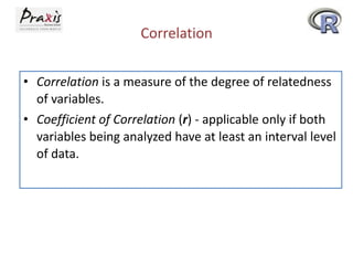
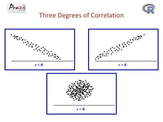
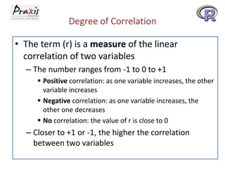
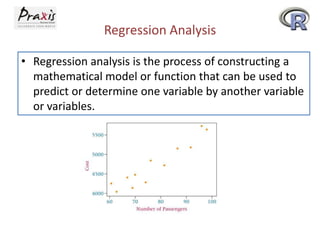
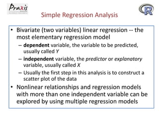
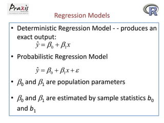
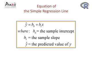
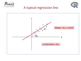
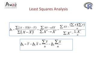
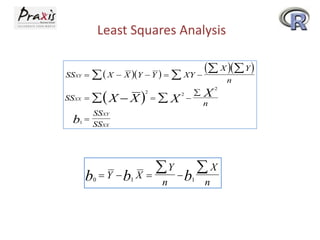
This document provides an overview of correlation and regression analysis concepts including: - Correlation measures the relationship between two variables while regression analysis is used to predict one variable based on another. - Simple linear regression involves predicting a dependent variable Y based on an independent variable X. - The least squares method is used to fit a regression line that minimizes the squared errors between observed and predicted Y values. 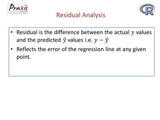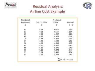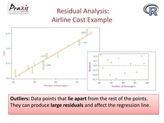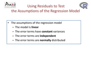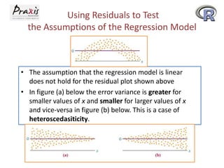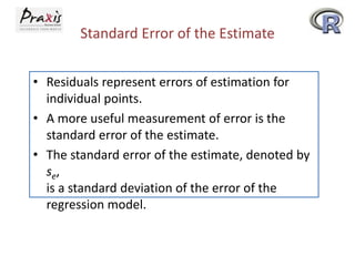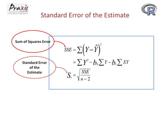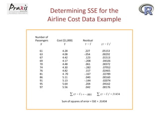- Residual analysis and other statistical measures like the standard error can be used to evaluate the fit of the regression model.

1. Correlation and Regression Analysis:
Learning Objectives
• Explain the purpose of regression analysis and the
meaning of independent versus dependent variables.
• Compute the equation of a simple regression line from a
sample of data, and interpret the slope and intercept of
the equation.
• Estimate values of Y to forecast outcomes using the
regression model.
• Understand residual analysis in testing the assumptions
and in examining the fit underlying the regression line.
• Compute a standard error of the estimate and interpret
its meaning.
• Compute a coefficient of determination and interpret it.

2. Correlation
• Correlation is a measure of the degree of relatedness
of variables.
• Coefficient of Correlation (r) - applicable only if both
variables being analyzed have at least an interval level
of data.

3. Three Degrees of Correlation
r<0
r>0
r=0

4. Degree of Correlation
• The term (r) is a measure of the linear
correlation of two variables
– The number ranges from -1 to 0 to +1
 Positive correlation: as one variable increases, the other
variable increases
 Negative correlation: as one variable increases, the
other one decreases
 No correlation: the value of r is close to 0
– Closer to +1 or -1, the higher the correlation
between two variables

5. Pearson Product-Moment
Correlation Coefficient

6. Regression Analysis
• Regression analysis is the process of constructing a
mathematical model or function that can be used to
predict or determine one variable by another variable
or variables.

7. Simple Regression Analysis
• Bivariate (two variables) linear regression -- the
most elementary regression model
– dependent variable, the variable to be predicted,
usually called Y
– independent variable, the predictor or explanatory
variable, usually called X
– Usually the first step in this analysis is to construct a
scatter plot of the data
• Nonlinear relationships and regression models
with more than one independent variable can be
explored by using multiple regression models

8. Regression Models
• Deterministic Regression Model - - produces an
exact output:
ˆ
y   0  1 x
• Probabilistic Regression Model
ˆ
y   0  1 x  
• 0 and 1 are population parameters
• 0 and 1 are estimated by sample statistics b0
and b1

9. Equation of
the Simple Regression Line

10. A typical regression line
Y
ϴ
X

11. Least Squares Analysis
• Least squares analysis is a process whereby a regression model
is developed by producing the minimum sum of the squared
error values
• The vertical distance from each point to the line is the error of
the prediction.
• The least squares regression line is the regression line that
results in the smallest sum of errors squared.

12. Least Squares Analysis
  X  X Y  Y    XY  nXY

b
 X n X
 X  X 
2
1
2
2


Y   X
b Y b X  n b n
0
1
1
 X  Y 
XY 
n
X
2


X
n
2

13. Least Squares Analysis
SSXY    X  X Y  Y   
SSXX  
b1 
X  X
2

X
 X  Y 
XY 
n
2


X
2
n
SSXY
SSXX
Y   X
b  Y b X  n b n
0
1
1

14. Airlines Cost Data include the costs and associated number of
passengers for twelve 500-mile commercial airline flights using
Boeing 737s during the same season of the year.
Number of
Passengers
61
63
67
69
70
74
76
81
86
91
95
97
Cost
($1,000)
4,280
4,080
4,420
4,170
4,480
4,300
4,820
4,700
5,110
5,130
5,640
5,560

15. Number of
Passengers
x
x2
61
63
67
69
70
74
76
81
86
91
95
97
x
Cost ($1,000)
y
4.28
4.08
4.42
4.17
4.48
4.30
4.82
4.70
5.11
5.13
5.64
5.56
3,721
3,969
4,489
4,761
4,900
5,476
5,776
6,561
7,396
8,281
9,025
9,409
= 930
y
= 56.69
x
2
= 73,764
xy
261.08
257.04
296.14
287.73
313.60
318.20
366.32
380.70
439.46
466.83
535.80
539.32
 xy
= 4,462.22

16. SS XY 
 XY 
SS XX 
X
b1 
b0 
2

 X Y
n
( X ) 2
n
 4,462 .22 
(930 )( 56 .69 )
 68 .745
12
(930 ) 2
 73,764 
 1689
12
SS XY
68 .745

 .0407
SS XX
1689
Y
n
 b1
X
n
ˆ
Y  1.57  .0407 X

56 .69
930
 (. 0407 )
 1.57
12
12

17. Residual Analysis

18. Residual Analysis:
Airline Cost Example
Number of
Passengers
X
61
63
67
69
70
74
76
81
86
91
95
97
Cost ($1,000)
Y
Predicted
Value
ˆ
Y
Residual
ˆ
Y Y
4.28
4.08
4.42
4.17
4.48
4.30
4.82
4.70
5.11
5.13
5.64
5.56
4.053
4.134
4.297
4.378
4.419
4.582
4.663
4.867
5.070
5.274
5.436
5.518
.227
-.054
.123
-.208
.061
-.282
.157
-.167
.040
-.144
.204
.042
 (Y  Yˆ )  .001

19. Residual Analysis:
Airline Cost Example
Outliers: Data points that lie apart from the rest of the points.
They can produce large residuals and affect the regression line.

20. Using Residuals to Test
the Assumptions of the Regression Model
• The assumptions of the regression model
– The model is linear
– The error terms have constant variances
– The error terms are independent
– The error terms are normally distributed

21. Using Residuals to Test
the Assumptions of the Regression Model
• The assumption that the regression model is linear
does not hold for the residual plot shown above
• In figure (a) below the error variance is greater for
smaller values of x and smaller for larger values of x
and vice-versa in figure (b) below. This is a case of
heteroscedasiticity.

22. Standard Error of the Estimate
• Residuals represent errors of estimation for
individual points.
• A more useful measurement of error is the
standard error of the estimate.
• The standard error of the estimate, denoted by
se,
is a standard deviation of the error of the
regression model.

23. Standard Error of the Estimate
Sum of Squares Error
SSE  
Standard Error
of the
Estimate
 

Y Y
2
  Y  b0  Y  b1  XY
2
SSE
Se  n  2

24. Determining SSE for the
Airline Cost Data Example
Number of
Passengers
X
Cost ($1,000)
Y
Residual
ˆ
Y Y
ˆ
(Y  Y ) 2
61
63
67
69
70
74
76
81
86
91
95
97
4.28
4.08
4.42
4.17
4.48
4.30
4.82
4 .70
5.11
5.13
5.64
5.56
.227
-.054
.123
-.208
.061
-.282
.157
-.167
.040
-.144
.204
.042
.05153
.00292
.01513
.04326
.00372
.07952
.02465
.02789
.00160
.02074
.04162
.00176
 (Y
ˆ
 Y )  .001
 (Y
ˆ
 Y ) 2 =.31434
Sum of squares of error = SSE = .31434

25. • The coefficient of determination is the proportion of
variability of the dependent variable (y) accounted
for or explained by the independent variable (x)
• The coefficient of determination ranges from 0 to 1.
• An r 2 of zero means that the predictor accounts for
none of the variability of the dependent variable
and that there is no regression prediction of y by x.
• An r 2 of 1 means perfect prediction of y by x and
that 100% of the variability of y is accounted for by
x.

26. SSYY  
Y Y   Y
2
 Y 

2
2
n
SSYY  exp lained var iation  un exp lained var iation
SSYY  SSR  SSE
SSR SSE
1

SSYY SSYY
SSR
2

r SSYY
SSE
 1
SSYY
SSE
 1
2
Y
2
Y  n
 

27. SSE  0.31434
 Y   270.9251 56.69  3.11209
 Y 
2
SSYY
2
n
SSE
r  1
SSYY
.31434
 1
3.11209
 .899
2
2
12
89.9% of the variability
of the cost of flying a
Boeing 737 is accounted for
by the number of passengers.

29. Exercise in R:
Linear Regression
Open URL: www.openintro.org
Go to Labs in R and select 7 - Linear Regression