STATE_SPACE_ANALYSIS.pdf

Introduction
• State space analysis is an powerful and modern approach for the design
and analysis of control systems.
• The conventional or old methods for the design and analysis of control
systems is based on transfer function method.
• The transfer function method for design and analysis had many drawbacks
such as..
– Transfer function is defined under zero initial conditions
– Applicable to LTI systems
– SISO systems
– Does not provide the information regarding internal state of
the system
• Initial conditions can be incorporated in the system design
• State equations are highly compatible for simulation on analog or digital
computers

Advantages of state variable analysis.
This can be applicable to
• Linear systems
• Non-linear system
• Time variant systems
• Time invariant systems
• Multiple input multiple output systems
• This gives idea about the internal state of the
system

Concept
The output not only depends on the input applied to the
system for t > t0, but also on the initial conditions at time t = t0
y(t) = y(t)│ t=t0 + y(t)│ t≥t0
` = ‫׬‬
−∞
t0
y t + ‫׬‬
t0
t
y(t)
= y(t0) + ‫׬‬
0
t
y(t)
The term y(t0) is called the state of the system.
The variable that represents this state of the system is called
the state variable
Output
SYSTEM
Input
r(t) y(t)

Definitions
State: The state of a dynamic system is the smallest set of
variables called state variables such that the knowledge of
these variables at time t = to (Initial condition), together
with the knowledge of input for t ≥ 𝑡0 , completely
determines the behavior of the system for any time 𝑡 ≥ 𝑡0 .
State Variables: A set of variables which describes the
system at any time instant are called state variables
State vector: A vector whose elements are the state
variables
State space: The n-dimensional space whose co-ordinate
axes consists of the x1 axis, x2 axis,.... xn axis, (where x1 , x2
,..... xn are state variables:) is called a state space.

Illustration
Consider the circuit shown in figure
i(t) = C
dvc
(t)
dt
Vc(t) =
1
𝐶
‫׬‬
−∞
t
i t dt
=
1
𝐶
‫׬‬
−∞
t0
i t dt +
1
C
‫׬‬
t0
t
i t dt
= Vc(t0) + Vc(t)
Vc(t0) = initial voltage across capacitor
The voltage across capacitor can be taken as a
state variable

Consider the circuit shown in figure
VL(t) = L
di(t)
dt
iL(t) =
1
𝐿
‫׬‬
−∞
t
VL(t)dt
=
1
𝐿
‫׬‬
−∞
t0
VL(t) dt +
1
L
‫׬‬
t0
t
VL(t) dt
= VL(t0) + VL(t)
VL(t0) = initial voltage across Inductor
The current through inductor can be taken as a
state variable
i(t)
L VL(t)

State Model
consider a multi-input & multi-output system is having
m inputs 𝑢1(𝑡) , 𝑢2(𝑡) ,…….𝑢m(𝑡)
p outputs 𝑦1(𝑡) , 𝑦2(𝑡) ,…….𝑦p(𝑡)
n state variables 𝑥1(𝑡) , 𝑥2(𝑡),…….𝑥𝑛(𝑡)
The different variables may be represented by the vectors as shown below
Input vector U(t) =
u1(t)
u2(t)
. .
um(t)
; Output vector Y(t) =
y1(t)
y2(t)
. .
yp(t)
State variable vector X(t) =
x1(t)
x2(t)
. .
xn(t)

State Equations
The state variable representation can be arranged
in the form of n number of first order differential
equations as shown below:
dx1
dt
= ሶ
x1 = f1(x1,x2,….xn ; u1,u2…..um)
dx2
dt
= ሶ
x2 = f1(x1,x2,….xn ; u1,u2…..um)
……
……
dxn
dt
= ሶ
xn = f1(x1,x2,….xn ; u1,u2…..um)
In vector notation, ሶ
X(t)= f(X(t),U(t))
Similarly the output vector Y(t) = f(X(t),U(t))

State Model of Linear System
The state model of a system consist of state equation and output
equation.
The state equation of a system is a function of state variables
and inputs.
For LTI systems, the first derivatives of state variables can be
expressed as a linear combination of sate variables and inputs
ሶ
x1 = a11x1+a12x2+----+a1nxn + b11u1+b12u2+---+b1mum
ሶ
x2 = a21x1+a22x2+----+a2nxn + b21u1+b22u2+---+b2mum
---
---
ሶ
xn = an1x1+an2x2+----+annxn + bn1u1+bn2u2+---+bnmum
where the coefficients aij and bij are constants

In the matrix form,
ሶ
x1
ሶ
x2
.
.
ሶ
xn
=
a11
a21
.
⋯
a1n
a2n
.
⋮ ⋱ ⋮
an1 ⋯ ann
x1
x2
. .
. .
xn
+
b11
b21
.
⋯
b1m
b2m
.
⋮ ⋱ ⋮
bn1 ⋯ bnm
u1
u2
. .
. .
um
Ẋ(t) = A X(t) + B U(t)……… state equation
where, A is state matrix of size (n×n)
B is the input matrix of size (n×m)
X(t) is the state vector of size (n×1)
U(t) is the input vector of size (m×1)

Output equation
The output at any time are functions of state
variables and inputs.
output vector, Y(t) = f(x(t), U(t))
Hence the output variables can be expressed as a
linear combination of state variables and inputs.
y1= c11x1+c12x2+----+c1nxn + d11u1+d12u2+---+d1mum
y2 = c21x1+c22x2+----+c2nxn + d21u1+d22u2+---+d2mum
---
---
yp = cp1x1+cp2x2+----+cpnxn + dp1u1+dp2u2+---+dpmum
where the coefficients cij and dij are constants

In the matrix form,
𝑦1
𝑦2
. .
. .
𝑦𝑝
=
c11
c21
.
⋯
c1n
c2n
.
⋮ ⋱ ⋮
cp1 ⋯ cpn
x1
x2
. .
. .
xn
+
d11
d21
.
⋯
d1m
d2m
.
⋮ ⋱ ⋮
dp1 ⋯ dpm
u1
u2
. .
. .
um
Y(t) = C X(t) + D U(t)………….. output equation
where, C is the output matrix of size (p×n)
D is the transmission matrix of size (p×m)
X(t) is the state vector of size (n×1)
Y(t) is the output vector of size (p×1)
U(t) is the input vector of size (m×1)

State Model
Ẋ(t) = A X(t) + B U(t) state equation
Y(t) = C X(t) + D U(t) output equation

Selection of state variables
• The state variables of a system are not unique.
• There are many choices for a given system
Guide lines:
1. For a physical systems, the number of state variables
needed to represent the system must be equal to the
number of energy storing elements present in the system
2. If a system is represented by a linear constant coefficient
differential equation, then the number of state variables
needed to represent the system must be equal to the
order of the differential equation
3. If a system is represented by a transfer function, then the
number of sate variables needed to represent the system
must be equal to the highest power of s in the
denominator of the transfer function.

State space Representation using Physical variables
• In state-space modeling of the systems, the
choice of sate variables is arbitrary.
• One of the possible choice is physical
variables.
• The state equations are obtained from the
differential equations governing the system

State Space Model
Consider the following series of the RLC circuit.
It is having an input voltage vi(t) and the current
flowing through the circuit is i(t).

• There are two storage elements (inductor and
capacitor) in this circuit. So, the number of the
state variables is equal to two.
• These state variables are the current flowing
through the inductor, i(t) and the voltage
across capacitor, vc(t).
• From the circuit, the output voltage, v0(t) is
equal to the voltage across capacitor, vc(t).

Y(t) = v0(t) = vc(t)
Apply KVL around the loop,
Vi(t) = R i(t) + L
di(t)
dt
+ vc(t)
ሶ
𝑖 𝑡 =
di(t)
dt
= -
R
L
i(t) -
1
L
vc(t) +
1
L
Vi(t)
The voltage across the capacitor is
vc(t) =
1
c
‫׬‬ i t dt
Differentiate the equation with respect to time,
ሶ
𝑣𝑐 𝑡 =
dvc
(t)
dt
=
i(t)
c
State vector, X =
i(t)
vc(t)
; Differential state vector, ሶ
X =
di(t)
dt
dvc
(t)
dt

Arrange the differential equations and output equation into standard
form of state space model as,
ሶ
X =
di(t)
dt
dvc
(t)
dt
=
−R
L
−1
L
1
C
0
i(t)
vc(t)
+
1
L
0
vi(t)
Y = 0 1
i(t)
vc(t)
Ẋ(t) = A X(t) + B U(t)
Y(t) = C X(t) + D U(t)
Here A =
−R
L
−1
L
1
C
0
; B =
1
L
0
; C = 0 1 ; D = [0]

Problem
Represent the electrical circuit shown by a state
model

Solution
Since there are three energy storing elements, choose
three state variables to represent the systems
The current through the inductors i1,i2 and voltage
across the capacitor vc are taken as state variables
Let the three sate variables be x1, x2 and x3 be related
to physical quantities as shown
Let, i1 = x1,
i2 = x2,
vc = x3

Applying KVL to loop 1,
L1
di1
(t)
dt
+ R1i1(t) + u(t) – vc(t) = 0
⟹ L1
dx1
(t)
dt
+ R1x1(t) + u(t) – x3(t) = 0
⟹ L1 ሶ
x1(t) + R1x1(t) + u(t) – x3(t) = 0
⟹ ሶ
x1(t) = -
R1
L1
x1(t) +
1
L1
x3(t) -
1
L1
u(t)-------(1)
Applying KVL to loop 2,
L2
di2
(t)
dt
+ R2i2(t) – vc(t) = 0
⟹ L2
dx2
(t)
dt
+ R2x2(t) – x3(t) = 0
⟹ L2 ሶ
x2(t) + R2x2(t) – x3(t) = 0
⟹ ሶ
x2(t) = -
R2
L2
x2(t) +
1
L2
x3(t) ------------------(2)

Applying KCL at node vc(t),
i1(t) + i2(t) + C
dvc
(t)
dt
= 0
⟹ x1(t) + x2(t) + C
dx3
(t)
dt
= 0
⟹ ሶ
x3(t) = -
1
C
x1(t) -
1
C
x2(t) --------------(3)
Putting 1, 2and 3 in matrix form,
ሶ
x1(t)
ሶ
x2(t)
ሶ
x3(t)
=
−
R1
L1
0
1
L1
0 −
R2
L2
1
L2
−
1
C
−
1
C
0
x1(t)
x2(t)
x3(t)
+
−
1
L1
0
0
u(t)
This is State Equation

y(t) = R2i2(t) = R2x2(t)
y(t) = 0 R2 0
x1(t)
x2(t)
x3(t)
This is output equation

Problem
Obtain the state model for a system represented
by an electrical system as shown in figure

Solution
Since there are two energy storage elements
present in the system, assume two state
variables to describe the system behavior.
Let the two state variables be x1 and x2 be
related to physical quantities as shown
Let v1(t) = x1(t)
v2(t) = x2(t)

Applying KCL at node v1(t),
v1
t −u(t)
R
+ C
dv1
(t)
dt
+
v1
t −v2
(t)
R
= 0
⟹
x1
t −u(t)
R
+ C
dx1
(t)
dt
+
x1
t −x2
(t)
R
= 0
⟹
2x1
t
R
-
u(t)
R
+ C ሶ
x1(t) -
x2
(t)
R
= 0
⟹ ሶ
x1(t) = -
2x1
t
RC
+
x2
(t)
RC
+
u(t)
RC
------------(1)

Applying KCL at node v2(t),
C
dv2
(t)
dt
+
v2
t −v1
(t)
R
= 0
⟹ C
dx2
(t)
dt
+
x2
t −x1
(t)
R
= 0
⟹ C ሶ
x2(t) -
x1
(t)
R
+
x2
t
R
= 0
⟹ ሶ
x2(t)=
x1
t
RC
-
x2
(t)
R𝐶
----------(2)

putting 1 and 2 in matrix form,
ሶ
x1(t)
ሶ
x2(t)
=
−2
RC
1
RC
1
RC
−1
RC
x1(t)
x2(t)
+
1
RC
0
u(t)
This is the state equation
The output of the circuit is given by
y(t) = v2(t)
= x2(t)
= 0 1
x1(t)
x2(t)
This is the output equation

Problem
Represent the electrical network by a state
equation

State representation using Phase variables
• The phase variables are defined as those particular
state variables which are obtained from one of the
system variables and its derivatives.
• Usually the variables used is the system output and
the remaining state variables are then derivatives of
the output.
• The state model using phase variables can be easily
determined if the system model is already known in
the differential equation or transfer function form.

Consider the following nth order linear differential equation relating the
output y(t) to the input u(t) of a system.
dn
y
dtn + 𝑎1
d𝑛−1𝑦
dt𝑛−1 + 𝑎2
d𝑛−2𝑦
dt𝑛−2 +-----+ 𝑎𝑛−1
dy
dt
+ 𝑎𝑛 𝑦 = u
Let us define the state variables as
𝑥1 = 𝑦
𝑥2 =
dy
dt
=
𝑑𝑥1
𝑑𝑡
𝑥3 =
d2
y
dt2 =
dẏ
dt
=
𝑑𝑥2
𝑑𝑡
⋮ ⋮ ⋮
𝑥𝑛 =
d𝑛−1𝑦
dt𝑛−1 =
𝑑𝑥𝑛−1
𝑑𝑡
From the above equations we can write
ሶ
x1 = 𝑥2
ሶ
x2 = 𝑥3
⋮ ⋮
ሶ
x𝑛−1 = 𝑥𝑛
ሶ
x𝑛 + 𝑎1𝑥𝑛 + …..+ 𝑎 𝑛−1𝑥2 +𝑎𝑛𝑥1 = 𝑢
ሶ
x𝑛 = − 𝑎𝑛𝑥1 − 𝑎 𝑛−1𝑥2……..−𝑎1𝑥𝑛 + 𝑢

writing the above state equation in vector matrix form,
ሶ
X(t) = AX(t) + Bu(t)
ሶ
x1
ሶ
x2
.
ሶ
x𝑛
=
0
0
⋯
0
0
⋮ ⋱ ⋮
−𝑎𝑛 ⋯ −𝑎1
x1
x2
.
x𝑛
+
0
0
.
1
[u]
Output equation can be written as
Y(t) = C X(t)= 1 0 0 . .
x1
x2
.
x𝑛

Problem
Construct a state model for a system characterized
by the differential equation,
d3
y
dt3 + 6
d2
y
dt2 + 11
dy
dt
+ 6y + u = 0
Also give the block diagram representation of the
state model
Solution: Let us choose y and their derivatives as
state variables. The system is governed by third
order differential equation, so the number of state
variables required are three.

Let the state variables x1, x2 and x3 are related to
phase variables as follows.
x1 = y
x2 =
dy
dt
= ሶ
x1
x3 =
d2
y
dt2 =
dx2
dt
= ሶ
x2
Put y = x1,
dy
dt
= x2,
d2
y
dt2 = x3 and
d3
y
dt3 = ሶ
x3 in the
given equation
∴ ሶ
x3+ 6x3 + 11x2 + 6x1 + u = 0
⟹ ሶ
x3 = - 6x1- 11x2 - 6x3 - u

The state equations are
ሶ
x1 = x2
ሶ
x2 = x3
ሶ
x3 = - 6x1- 11x2 - 6x3 - u
Arranging the state equations in the matrix form,
ሶ
x1
ሶ
x2
ሶ
x3
=
0 1 0
0 0 1
−6 −11 −6
x1
x2
x3
+
0
0
−1
[u]
Here y = output
But y = x1
∴ The output equation is, y = [1 0 0]
x1
x2
x3

The block diagram for the state model is

Problem
Represent the differential equation given below
in a state model
d3
y
dt3 +
d2
y
dt2 + 6
dy
dt
+7y = 2u(t)
Solution:
Since, the given equation is a third-order
differential equation, choose three state
variables to represent the system

Let y(t) = x1(t)
ሶ
y(t) = x2(t)
ሷ
y(t) = x3(t)
where x1(t), x2(t), x3(t) are the state variables of
the system.
y(t) = x1(t)
ሶ
y(t) = x2(t) = ሶ
x1(t) -----------(1)
ሷ
y(t) = x3(t) = ሶ
x2(t) -----------(2)

From the given diff. equation,
d3
y
dt3 +
d2
y
dt2 + 6
dy
dt
+7y = 2u(t)
ഺ
𝑦 (t) + ሷ
𝑦(t) + 6 ሶ
𝑦(t) +7y = 2u(t)
ሶ
x3(t) + x3(t) + 6 x2(t) + 7 x1(t) = 2u(t)
ሶ
x3(t) = -7 x1(t) - 6 x2(t) - x3(t) + 2u(t) ------(3)
ሶ
x2(t) = x3(t) ------(2)
ሶ
x1(t) = x2(t) ------(1)

Putting the above equations in matrix form,
ሶ
x1
ሶ
x2
ሶ
x3
=
0 1 0
0 0 1
−7 −6 −1
x1
x2
x3
+
0
0
2
u(t)
This is the state equation
The output expression is y(t) = x1(t)
= 1 0 0
x1
x2
x3
This is the output equation

Problem
Obtain the state model for the signal flow graph
given below:

Problem
Obtain the state model of the system whose transfer
function is given by
Y(s)
U(s)
=
24
𝑠3
+9𝑠2
+26𝑠+24
Solution:
Y(s)
U(s)
=
24
𝑠3
+9𝑠2
+26𝑠+24
Cross-multiplying yields
[s3 + 9s2 + 26s + 24] Y(s) = 24 U(s)
s3 Y(s) + 9s2 Y(s) + 26sY(s) + 24 Y(s) = 24U(s)
Taking inverse Laplace transforms,
d3
y(t)
dt3 + 9
d2
y(t)
dt2 + 26
dy(t)
dt
+ 24 y(t) = 24u(t)
ഺ
y(t) + 9 ሷ
y(t) + 26 ሶ
y(t) + 24 y(t) = 24u(t)

Choosing the state variables as successive derivatives
x1(t) = y(t)
x2(t) = ሶ
y(t)
x3(t) = ሷ
y(t)
x1(t) = y(t)
ሶ
x1(t) = x2(t) = ሶ
y(t) -----(1)
ሶ
x2(t) = x3(t) = ሷ
𝑦(t) -----(2)
ሶ
x3(t) = ഺ
𝑦(t)
ഺ
y(t) + 9 ሷ
y(t) + 26 ሶ
y(t) + 24 y(t) = 24u(t)
ሶ
x3(t) + 9x3(t) + 26x2(t) + 24x1(t) = 24u(t)
ሶ
x3(t) = - 24x1(t) - 26x2(t) - 9x3(t) + 24u(t)------(3)

Putting equations 1, 2 and 3 in matrix form,
ሶ
x1
ሶ
x2
ሶ
x3
=
0 1 0
0 0 1
−24 −26 −9
x1
x2
x3
+
0
0
24
[u]
The output expression is y(t) = x1(t)
= 1 0 0
x1
x2
x3

Matlab
Obtain the state model of the system whose
transfer function is given by
Y(s)
U(s)
=
24
𝑠3
+9𝑠2
+26𝑠+24
using Matlab

Problem
Obtain the state model of the system whose transfer function is
given by
Y(s)
U(s)
=
1
s2
+s+1
Solution:
Y(s)
U(s)
=
1
s2
+s+1
⟹ (s2 + s + 1)Y(s) = U(s)
s2 Y(s) + s Y(s) + Y(s) = U(s)
Taking inverse Laplace transform on both sides,
d2
y(t)
dt2 +
dy(t)
dt
+ y(t) = u(t)
Let y(t) = x1
𝑑𝑦(𝑡)
𝑑𝑡
= x2 = ሶ
x1 and u(t) = u

Then the state equation is, ሶ
x2 = -x1-x2+u
The output equation is, y(t) = y = x1
The state space model is
ሶ
x =
ሶ
x1
ሶ
x2
= =
0 1
−1 − 1
x1
x2
+
0
1
[u]
Y= 1 0
x1
x2

Problem
s2
+7s+2
s3
+9s2
+26s+24
Solution:
Y(s)
U(s)
=
s2
+7s+2
s3
+9s2
+26s+24
Y(s)
U(s)
=
Y(s)
C(s)
x
C(s)
U(s)
Y(s)
C(s)
= s2 + 7s + 2 --------(1)
C(s)
U(s)
=
1
s3
+9s2
+26s+24
-------(2)

Consider equation (2),
C(s)
U(s)
=
1
s3
+9s2
+26s+24
Cross-multiplying on both sides,
[s3 + 9s2 + 26s + 24] C(s) = U(s)
s3 C(s) + 9s2 C(s) + 26s C(s) + 24 C(s) = U(s)
Taking inverse Laplace transform,
d3
c(t)
dt3 + 9
d2
c(t)
dt2 + 26
dc(t)
dt
+ 24 c(t) = u(t)
ഺ
c (t) + 9 ሷ
c(t) + 26 ሶ
c(t) +24 c(t) = u(t)
x1(t) = c(t)
ሶ
x1(t) = x2(t) = ሶ
c(t) -----(3)
ሶ
x2(t) = x3(t) = ሷ
c(t) -----(4)
ሶ
x3(t) = ഺ
c(t)

ഺ
c (t) + 9 ሷ
c(t) + 26 ሶ
c(t) + 24c(t) = u(t)
ሶ
x3(t) + 9 x3(t) + 26x2(t) + 24x1(t) = u(t)
ሶ
x3(t) = - 24x1(t) - 26x2(t) - 9 x3(t) + u(t) -----(5)
Putting equations 3, 4 and 5 in matrix form,
ሶ
x1
ሶ
x2
ሶ
x3
=
0 1 0
0 0 1
−24 −26 −9
x1
x2
x3
+
0
0
1
[u]

Consider equation (1),
Y(s)
C(s)
= s2 + 7s + 2
Y(s) = [s2 + 7s + 2]C(s)
Y(s) = s2C(s) + 7sC(s) + 2C(s)
Taking inverse Laplace transform,
y(t) = ሷ
c(t) + 7 ሶ
c(t) +2c(t)
y(t) = 2x1(t) + 7x2(t) + x3(t)
y(t) = 2 7 1
x1
x2
x3

Matlab
s2
+7s+2
s3
+9s2
+26s+24
using
Matlab

Problem
A feedback system has a closed-loop transfer
function
Y(s)
U(s)
=
2(s+5)
(s+2)(s+3)(s+4)
Solution:
Y(s)
U(s)
=
2(s+5)
(s+2)(s+3)(s+4)
By partial fraction expansion,
Y(s)
U(s)
=
2(s+5)
(s+2)(s+3)(s+4)
=
A
(s+2)
+
B
(s+3)
+
C
(s+4)
Solving for A, B and C
A = 3; B = - 4; C = 1

Y(s)
U(s)
=
2(s+5)
(s+2)(s+3)(s+4)
=
3
(s+2)
-
4
(s+3)
+
1
(s+4)
-----(1)
=
3
s(1+2/s)
-
4
s(1+3/s)
+
1
s(1+4/s)
=
1
s
(1+
1
s
∗2)
x 3 -
1
s
(1+
1
s
∗3)
x 4 +
1
s
(1+
1
s
∗4)
∴ Y s = [
1
s
(1+
1
s
∗2)
x 3 -
1
s
(1+
1
s
∗3)
x 4 +
1
s
(1+
1
s
∗4)
]u(s)
= [
1
s
(1+
1
s
∗2)
x 3]U(s) - [
1
s
(1+
1
s
∗3)
x 4] U(s) + [
1
s
(1+
1
s
∗4)
]u(s)

The equation can be represented by the block
diagram as shown
Assign state variables at the output of the
integrators as shown.
At the input of the integrators , first derivative of
the state variables are present.
The state equations are formed by adding all the
incoming signals to the integrator and equating
to the corresponding first derivative of state
variables.

The state equations are
ሶ
x1 = -2x1 + u
ሶ
x2 = -3x2 + u
ሶ
x3 = -4x3 + u

The output equation is
y = 3x1- 4x2 + x3
The State model is given by,
ሶ
x1
ሶ
x2
ሶ
x3
=
−2 0 0
0 −3 0
0 0 −4
x1
x2
x3
+
1
1
1
u
Y = 3 − 4 1
x1
x2
x3

Matlab
Find the state model for the transfer function
2(s+5)
(s+2)(s+3)(s+4)
using Matlab

Solution of State Equation
S-Domain:
The State equation of nth order system is given by,
ሶ
x(t) = A X(t) + BU(t); X(0) = X0 = initial condition vector
Taking Laplace transforms on both sides,
S X(s)-X(0) = A X(s) + B U(s)
X(s)[sI-A] = X(0) + B U(s) where I = unit matrix
X(s) = [sI-A]-1 X(0) + [SI-A]-1 B U(s) --------------(1)
Taking inverse Laplace transforms on both sides,
X(t) = L-1 [sI-A]-1 X(0) + L-1 [SI-A]-1 B U(s)
where L-1 [sI-A]-1 = ∅(t) = state transition matrix
[sI-A]-1 = ∅(s) = Resolvent matrix
The solution of state equation is,
X(t) = ∅(t) X(0) + L-1 [∅(s). B U(s)]

The output equation is,
y(t) = C x(t) + D u(t)
Taking Laplace transforms on both sides,
Y(s) = C X(s) + D U(s)
From equation (1), X(s) = [sI-A]-1 X(0) + [SI-A]-1 B U(s)
= C{[sI-A]-1 X(0) + [SI-A]-1 B U(s)} + D U(s)
= C[sI-A]-1 X(0) + C [SI-A]-1 B U(s) + D U(s)
For zero initial conditions, X(0) = 0
∴ Y(s) = C [SI-A]-1 B U(s) +D U(s)
= {C [SI-A]-1 B +D} U(s)
The transfer function =
Y(s)
U(s)
= C [SI-A]-1 B + D

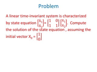
Problem
A state variable description of a system is given
by the matrix equation,
ሶ
X =
−1 0
1 −2
X +
1
0
u
Y = [ 1 1] X
Find (i) The Transfer function
(ii) The State transition matrix
(iii) State diagram

Solution
The state model is given by
ሶ
X = A X + B U
Y = C X + D U
From the given problem,
A =
−1 0
1 −2
B =
1
0
C = [ 1 1]
(i) The transfer function =
Y(s)
U(s)
= C [SI-A]-1 B + D
Here D =0
∴
Y(s)
U(s)
= C [SI-A]-1 B

[sI-A] = s
1 0
0 1
-
−1 0
1 −2
=
s 0
0 s
-
−1 0
1 −2
=
s + 1 0
−1 s + 2
[SI-A]-1 =
Adj A
Det A
=
s + 2 0
1 s + 1
1
(s+1)(s+2)
Y(s)
U(s)
= C [SI-A]-1 B
= [1 1]
s + 2 0
1 s + 1
{
1
(s+1)(s+2)
}
1
0
= {
1
(s+1)(s+2)
} [1 1]
s + 2 0
1 s + 1
1
0

Y(s)
U(s)
= {
1
(s+1)(s+2)
} [1 1]
s + 2
1
= {
1
(s+1)(s+2)
} [s+3]
=
s+3
(s+1)(s+2)
(ii) State transition matrix = ∅(t) = L-1 [sI-A]-1
[SI-A]-1 =
s + 2 0
1 s + 1
1
(s+1)(s+2)
=
s+2
(s+1)(s+2)
0
(s+1)(s+2)
1
(s+1)(s+2)
s+1
(s+1)(s+2)

[SI-A]-1 =
1
(s+1)
0
1
(s+1)(s+2)
1
(s+2)
∅(t) = L-1 [sI-A]-1
= L-1
1
(s+1)
0
1
(s+1)(s+2)
1
(s+2)
= L-1
1
(s+1)
0
1
(s+1)
−
1
(s+2)
1
(s+2)
= e−t 0
e−t
− e−2t
e−2t

(iii) State Diagram:
The state equation is,
ሶ
x1 = - x1 + u(t)
ሶ
x2 = x1 – 2x2
The output equation is y = x1 + x2

Matlab
Find the transfer function using Matlab

Problem
The state equation of a LTI system is given as
ሶ
x =
0 5
−1 −2
X +
1
1
u and y = [1 1] X
Determine (i) State transition matrix
(ii) The transfer function
(iii) State diagram

Solution
From the given system,
A =
0 5
−1 −2
B=
1
1
C= [1 1]
(i) The State transition matrix ,
∅(t) = L-1 [sI-A]-1
[sI – A] = s
1 0
0 1
-
0 5
−1 −2
=
s −5
1 s + 2
[sI-A]-1 =
s + 2 5
−1 s
1
s s+2 +5
=
s+2
s s+2 +5
5
s s+2 +5
−1
s s+2 +5
s
s s+2 +5

=
s+1+1
s+1 2
+22
5
s+1 2
+22
−1
s+1 2
+22
s
s+1 2
+22
∅(t) = L−1 [sI−A]−1
= L-1
s+1+1
s+1 2
+22
5
s+1 2
+22
−1
s+1 2
+22
s+1−1
s+1 2
+22
=
e−t cos 2t +
1
2
e−t sin 2t
5
2
e−t sin 2t
−
1
2
e−t sin 2t e−t cos 2t −
1
2
e−t sin 2t

(ii) The transfer function
Y(s)
U(s)
= C [SI-A]-1 B
= [1 1]
s + 2 5
−1 s
1
s s+2 +5
1
1
=
1
s s+2 +5
[1 1]
S + 7
S − 1
=
2S+6
s s+2 +5

Problem
Find the transfer function of a state model of a
system given by ,
ሶ
x =
0 1 0
0 0 1
−1 −2 −3
X +
0 0
1 0
0 1
u1
u2
and
y1
y2
=
1 0 0
0 0 1
X

Solution
From the given system,
A =
0 1 0
0 0 1
−1 −2 −3
; B =
0 0
1 0
0 1
;C =
1 0 0
0 0 1
[sI-A] = s
1 0 0
0 1 0
0 0 1
-
0 1 0
0 0 1
−1 −2 −3
=
s −1 0
0 s −1
1 2 s + 3

∴ [sI-A]-1 =
(s + 2)(s + 1) s + 3 1
−1 s(s + 3) s
−s −(2s + 1) s2
1
s3
+3s2
+2s+1
The transfer function of the system is given by
Y(s)
U(s)
= C [SI-A]-1 B
=
1 0 0
0 0 1
(s + 2)(s + 1) s + 3 1
−1 s(s + 3) s
−s −(2s + 1) s2
1
s3
+3s2
+2s+1
0 0
1 0
0 1
=
1 0 0
0 0 1
s + 3 1
s(s + 3) s
− 2s + 1 s2
1
s3
+3s2
+2s+1
=
s + 3 1
− 2s + 1 s2
1
s3
+3s2
+2s+1

Problem
A linear time-invariant system is characterized
by state equation
ሶ
x1
ሶ
x2
=
1 0
1 1
x1
x2
. Compute
the solution of the state equation , assuming the
initial vector X0 =
1
0

Solution
From the given system, A =
1 0
1 1
The solution of state equation is,
X(t) = L-1 [sI-A]-1 X(0) + L-1 [SI-A]-1 B U(s)
Here U= 0
∴ X(t) = L-1 [sI-A]-1 X(0)
[sI – A] = s
1 0
0 1
-
1 0
1 1
=
s − 1 0
−1 s − 1
[sI-A]-1 =
s − 1 0
1 s − 1
1
s−1 2

[sI-A]-1 =
s − 1 0
1 s − 1
1
s−1 2
=
1
s−1
0
1
s−1 2
1
s−1
X(t) = L-1 [sI-A]-1 X(0)
= L-1
1
s−1
0
1
s−1 2
1
s−1
1
0
= et
0
tet
et
1
0
= et
tet

Solution of state equation (Time Domain)
ሶ
x(t) = A x(t) + B u(t) X(0) = x0
ሶ
x(t) - A x(t) = B u(t)
pre-multiplying both sides by e−At
e−At[ ሶ
x(t) - A x(t)] = e−At B u(t) ----------------(1)
Consider,
𝑑
𝑑𝑡
{e−At x(t)} = e−At ሶ
x(t) - A e−At x(t)]
= e−At
[ ሶ
x(t) - A x(t)]
∴ equation (1) =
𝑑
𝑑𝑡
{e−At
x(t)} = e−At
B u(t)
Integrating with respect to t
‫׬‬0
t d
dt
{e−At x(t)} dt = ‫׬‬0
t
[e−Aτ B u(τ)]dτ
e−At x(t) – x(0) = ‫׬‬
0
𝑡
[e−Aτ B u(τ)]d𝜏

Pre-multiplying both sides by eAt,
eAt
[e−At
x(t) – x(0)] = eAt
[‫׬‬0
𝑡
e−Aτ
B u(τ)d𝜏]
x(t) = eAt
[x(0) + ‫׬‬0
t
e−Aτ
B u(τ)dτ]
= eAt
x(0) + ‫׬‬0
t
[eA(t−τ) B u(τ)]dτ
x(t) = ∅ t x(0) + ‫׬‬0
t
∅(t−τ) B u(τ) dτ
if the initial time is t = t0, the solution of state equation
becomes,
x(t) = ∅ t − t0 x(t0) + ‫׬‬0
t
∅(t−τ) B u(τ)dτ

Properties of state transition matrix
∅(t) = eAt = L-1 [sI-A]-1
1. ∅(0) = I
2. ∅-1(t) = ∅(-t)
3. ∅(t2-t1) ∅(t1-t0) = ∅(t2-t0) for any t2, t1, t0
4. [∅(t)]k = ∅(kt)
5. ∅(t1+t2) = ∅(t1) ∅(t2) = ∅(t2) ∅(t1)

Problem
Compute the State transition matrix by infinite
series method A =
0 1
−1 −2
Solution: For the given system matrix A, the state
transition matrix is,
∅ (t) = eAt
= I + At +
At 2
2!
+
At 3
3!
+------
A =
0 1
−1 −2
A2 = A. A =
0 1
−1 −2
.
0 1
−1 −2
=
−1 −2
2 3
A3 = A2.A =
−1 −2
2 3
.
0 1
−1 −2
=
2 3
−3 −4

∅(t) = I + At +
At 2
2!
+
At 3
3!
+---
=
1 0
0 1
+
0 1
−1 −2
t +
−1 −2
2 3
t2
2!
+
2 3
−3 −4
t3
3!
+- -
=
1 −
t2
2
+
t3
3
+ ⋯ t − t2 +
t3
2
+ ⋯
−t + t2 −
t3
2
+ ⋯ 1 − 2t +
3t2
2
+ ⋯
= e−t
+ te−t
te−t
−te−t e−t − te−t

Problem
Find the state transition matrix by infinite series
method for the system matrix A =
1 1
0 1
Solution: For the given system matrix A, the
state transition matrix is,
∅ (t) = eAt
= I + At +
At 2
2!
+
At 3
3!
+------
A =
1 1
0 1
A2 = A.A =
1 1
0 1
.
1 1
0 1
=
1 2
0 1

A3 = A2. A =
1 2
0 1
.
1 1
0 1
=
1 3
0 1
∅(t) = I + At +
At 2
2!
+
At 3
3!
+ ---
=
1 0
0 1
+
1 1
0 1
t +
1 2
0 1
t2
2!
+
1 3
0 1
t3
3!
+ ---
=
1 + t +
t2
2!
+
t3
3!
+ ⋯ t + t2 +
t3
2
+ ⋯
0 1 + t +
t2
2!
+
t3
3!
+. .
= et
tet
0 et

References
1. Control Engineering by Nagrath & Gopal, New
Age International Publishers
2. Engineering control systems - Norman S. Nise,
John WILEY & sons , fifth Edition
3. Modern control Engineering-Ogata, Prentice
Hall
4. Automatic Control Systems- B.C Kuo, John
Wiley and Sons

STATE_SPACE_ANALYSIS.pdf

Recommended

Recommended

More Related Content

What's hot

What's hot (20)

Similar to STATE_SPACE_ANALYSIS.pdf

Similar to STATE_SPACE_ANALYSIS.pdf (20)

Recently uploaded

Recently uploaded (20)

STATE_SPACE_ANALYSIS.pdf