
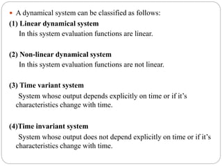
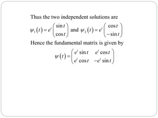
![(5) Discrete time system
The state variable representing the current state of discrete time system
(digital) is where is discrete point at which system is being
evaluated. The discrete time state equations are
which describe the next state of system
with respect to current state and inputs of system.
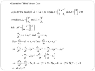
(6) Continuous time system
The state variable representing the current state of a continuous time
system (analog) is and the continuous time state equations are
which describe the next state of system with respect to current state
and inputs of system.
x n
1 [ ] [ ]x n Ax n Bu n
1x n
[ ]u n
x t
dx t
Ax t Bu t
dt
dx t
dt](https://image.slidesharecdn.com/pkpcontrollabilityoflineardynamicalsystem-160809125127/85/Controllability-of-Linear-Dynamical-System-5-320.jpg)
![
1 1
0 0 1 0 0 1
1
2 2
2
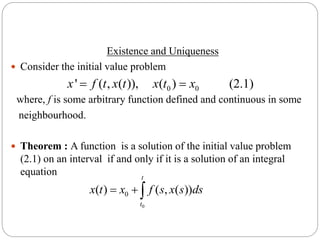
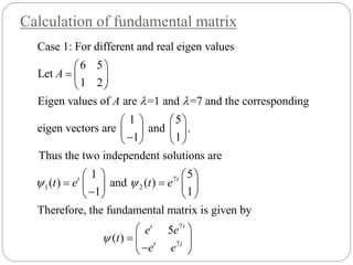
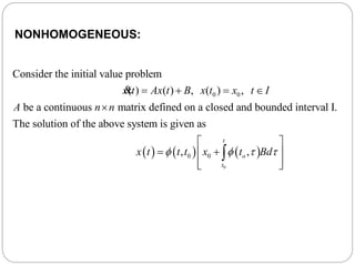
We can find the controller ( ) as follows
( ) ( , ) ( , )[ ( , ) ]
5.7454 2.7278 0 10 0
= 1 1
2.7278 1.3697 0 10 0
5.7454 2.
=
T T
t
t
t t
u t
u t B t t W t t X t t X
e e
e e
e e
2
2
7278 2.7183
2.7278 1.3697 7.3891
4.5383
=
2.7059
( )= 4.5383 2.7059
t t
t t
e e
u t e e
](https://image.slidesharecdn.com/pkpcontrollabilityoflineardynamicalsystem-160809125127/85/Controllability-of-Linear-Dynamical-System-21-320.jpg)
![
0 0 0
0
2
2 2
0
2
2
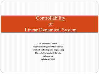
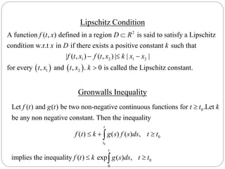
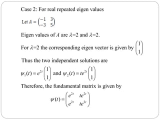
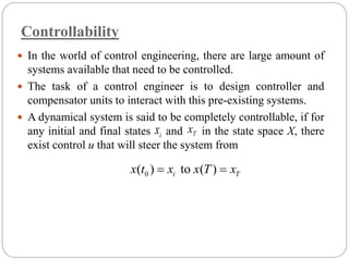
We can find the solution ( ) as follows
( ) ( , )[ ( , ) ]
0 10 0
= 4.5383 2.7059
0 10 0
0 4.5383 2.7059
=
0
t
tt
t
t
t
X t
X t t t X t Bu d
e e
e e d
e e
e e e
e
3
3 4
0
2 3
2 3 4
0
2 3
2 3 4
4.5383 2.7059
0 2.2691 0.9020
=
0 1.5128 0.6765
0 2.2691 0.9020 1.3671
=
0 1.5128 0.6765 0.8363
t
tt
t
t t t
t t t
d
e e
e e e
e e e
e e e
e e e
X
2
2 2
2.2691 0.9020 1.3671
( )=
1.5128 0.6765 0.8363
t t t
t t t
e e e
t
e e e
](https://image.slidesharecdn.com/pkpcontrollabilityoflineardynamicalsystem-160809125127/85/Controllability-of-Linear-Dynamical-System-22-320.jpg)
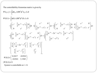
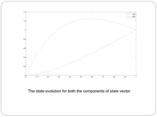
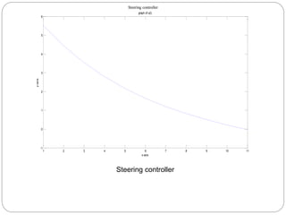

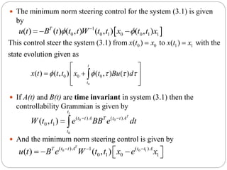
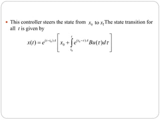
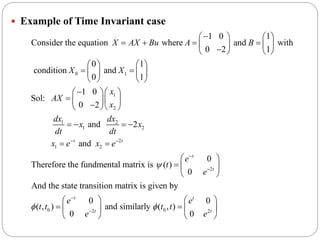
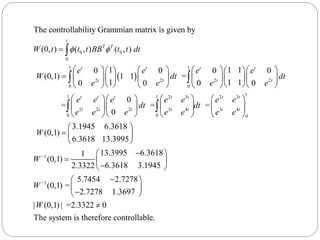
The document discusses linear dynamical systems and controllability of linear systems. It defines dynamical systems as mathematical models describing the temporal evolution of a system. Linear dynamical systems are ones where the evaluation functions are linear. Controllability refers to the ability to steer a system from any initial state to any final state using input controls. The document provides the definition of controllability for linear time-variant systems using the controllability Gramian matrix. It also gives the formula for the minimum-norm control input that can steer the system between any two states. An example of checking controllability for a time-invariant linear system is presented.