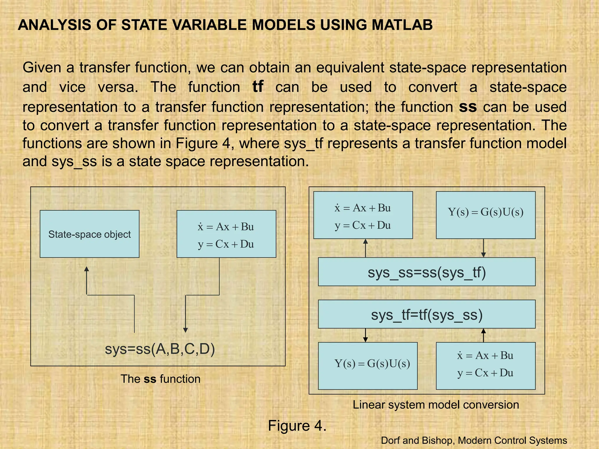
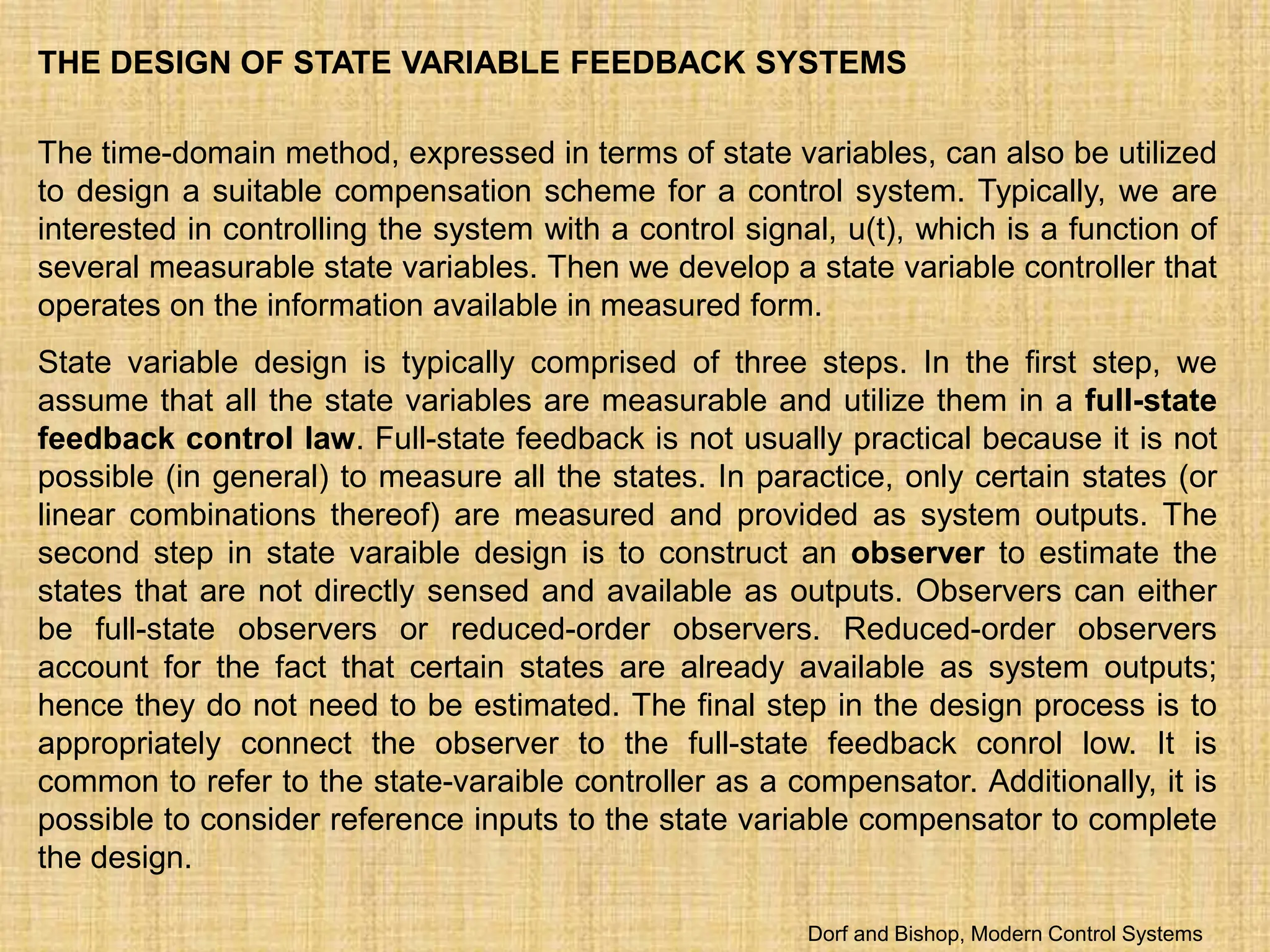
The document discusses state variable models for physical systems described by ordinary differential equations, demonstrating how to derive first-order equations and matrix forms suitable for computer analysis. It details the role of state variables in predicting the future state of a system based on current conditions and inputs, illustrating with examples such as spring-mass-damper systems and RLC circuits. The text emphasizes the usefulness of state-space representation in modern control systems, including transfer function derivation and analysis techniques using MATLAB.

1. STATE VARIABLE MODELS
Dr.Ziad Saeed Mohammed
2019-2020

2. STATE VARIABLE MODELS
We consider physical sytems described by nth-order ordinary differential
equation. Utilizing a set of variables, known as state variables, we can
obtain a set of first-order differential equations. We group these first-order
equations using a compact matrix notation in a model known as the state
variable model.
The time-domain state variable model lends itself readily to computer
solution and analysis. The Laplace transform is utilized to transform the
differential equations representing the system to an algebraic equation
expressed in terms of the complex variable s. Utilizing this algebraic
equation, we are able to obtain a transfer function representation of the
input-output relationship.
With the ready availability of digital computers, it is convenient to consider
the time-domain formulation of the equations representing control system.
The time domain techniques can be utilized for nonlinear, time varying, and
multivariable systems.
Dorf and Bishop, Modern Control Systems

3. A time-varying control system is a system for which one or more of the
parameters of the system may vary as a function of time.
For example, the mass of a missile varies as a function of time as the fuel is
expended during flight. A multivariable system is a system with several input
and output.
The State Variables of a Dynamic System:
The time-domain analysis and design of control systems utilizes the concept
of the state of a system.
The state of a system is a set of variables such that the knowledge of these
variables and the input functions will, with the equations describing the
dynamics, provide the future state and output of the system.

4. For a dynamic system, the state of a system is described in terms of a set of
state variables
)]
t
(
x
)
t
(
x
)
t
(
x
[ n
2
1 
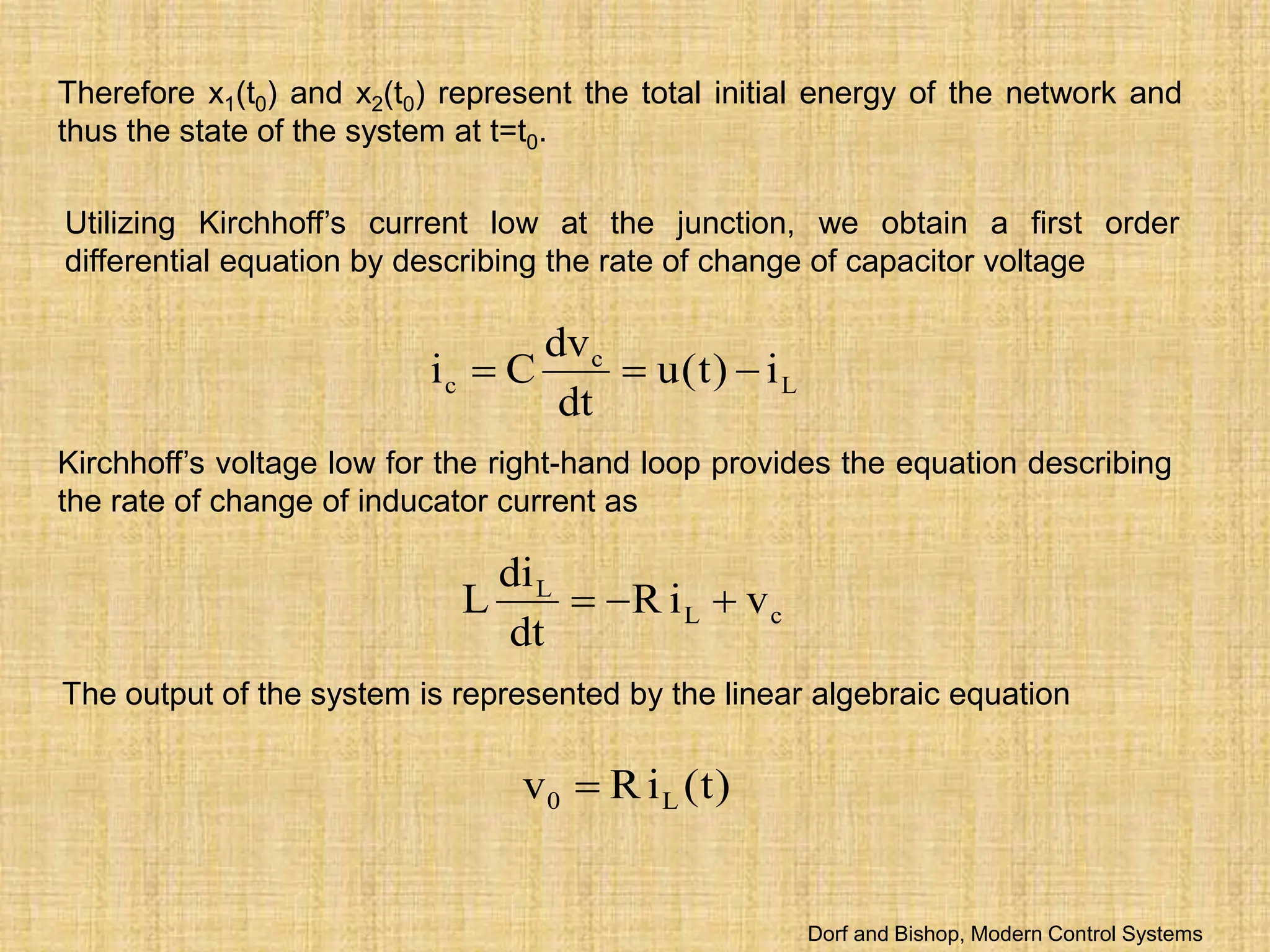
The state variables are those variables that determine the future behavior of
a system when the present state of the system and the excitation signals are
known. Consider the system shown in Figure 1, where y1(t) and y2(t) are the
output signals and u1(t) and u2(t) are the input signals. A set of state
variables [x1 x2 ... xn] for the system shown in the figure is a set such that
knowledge of the initial values of the state variables [x1(t0) x2(t0) ... xn(t0)] at
the initial time t0, and of the input signals u1(t) and u2(t) for t˃=t0, suffices to
determine the future values of the outputs and state variables.
System
Input Signals
u1(t)
u2(t)
Output Signals
y1(t)
y2(t)
System
u(t)
Input
x(0) Initial conditions
y(t)
Output
Figure 1. Dynamic system.

5. The state variables describe the future response of a system, given the
present state, the excitation inputs, and the equations describing the
dynamics.
A simple example of a state variable is the state of an on-off light switch.
The switch can be in either the on or the off position, and thus the state of
the switch can assume one of two possible values. Thus, if we know the
present state (position) of the switch at t0 and if an input is applied, we are
able to determine the future value of the state of the element.
The concept of a set of state variables that
represent a dynamic system can be illustrated in
terms of the spring-mass-damper system shown
in Figure 2. The number of state variables chosen
to represent this system should be as small as
possible in order to avoid redundant state
variables. A set of state variables sufficient to
describe this system includes the position and the
velocity of the mass.
k c
m
y(t) u(t)
Figure 2. 1-dof system.

6. dt
)
t
(
dy
)
t
(
x
)
t
(
y
)
t
(
x
2
1


y
y
c
y
)
t
(
u
W
,
y
k
2
1
E
,
y
m
2
1
E 2
2
2
1 





 

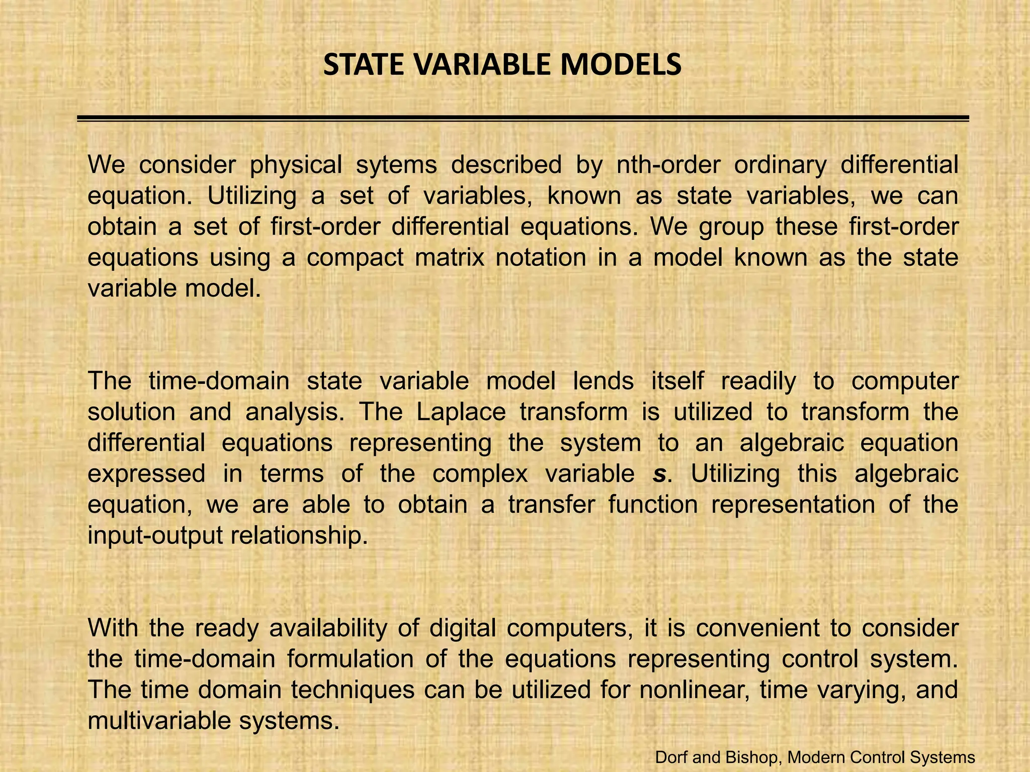
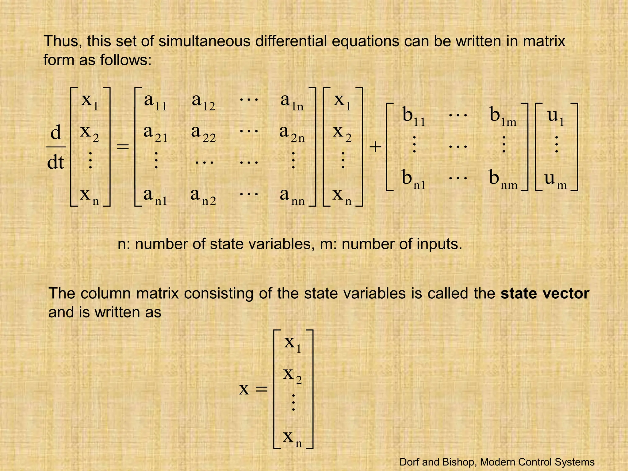
Kinetic and Potential energies, virtual work.
Therefore we will define a set of variables as [x1 x2], where
Lagrange’s equation    
y
2
1
2
1
Q
y
E
E
y
E
E
dt
d

















2
1 E
E
L 

Lagrangian of the system is expressed as Generalized Force
)
(
)
(
1
2
2
2
2
t
u
x
k
x
c
dt
dx
m
t
u
y
k
dt
dy
c
dt
y
d
m






Equation of motion in terms of state variables.
We can write the equations that describe the behavior of the spring-mass-
damper system as the set of two first-order differential equations.

7. )
t
(
u
m
1
x
m
k
x
m
c
dt
dx
x
dt
dx
1
2
2
2
1





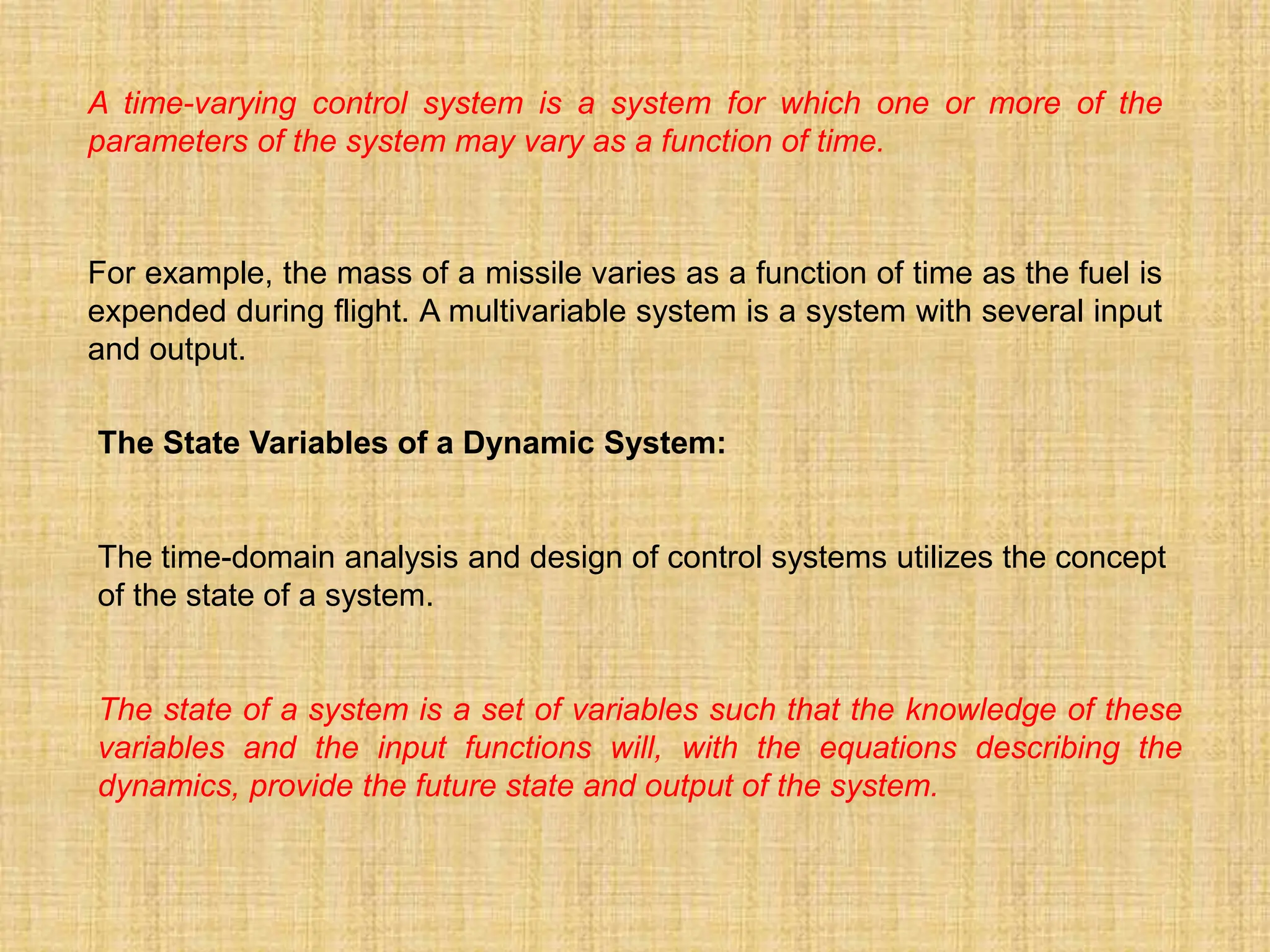
This set of difefrential equations
describes the behavior of the state of
the system in terms of the rate of
change of each state variables.
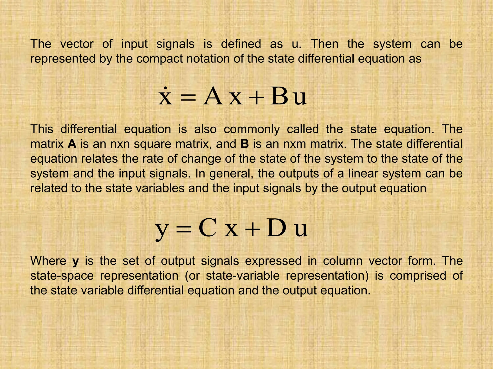
As another example of the state variable characterization of a system, consider the
RLC circuit shown in Figure 3.
u(t)
Current
source
L
C
R
Vc
Vo
iL
ic
  2
c
2
c
2
2
L
1 v
C
2
1
dt
i
C
2
1
E
,
i
L
2
1
E 

 
The state of this system can
be described in terms of a set
of variables [x1 x2], where x1
is the capacitor voltage vc(t)
and x2 is equal to the inductor
current iL(t). This choice of
state variables is intuitively
satisfactory because the
stored energy of the network
can be described in terms of
these variables.
Figure 3

8. Therefore x1(t0) and x2(t0) represent the total initial energy of the network and
thus the state of the system at t=t0.
Utilizing Kirchhoff’s current low at the junction, we obtain a first order
differential equation by describing the rate of change of capacitor voltage
L
c
c i
)
t
(
u
dt
dv
C
i 


Kirchhoff’s voltage low for the right-hand loop provides the equation describing
the rate of change of inducator current as
c
L
L
v
i
R
dt
di
L 


The output of the system is represented by the linear algebraic equation
)
t
(
i
R
v L
0 
Dorf and Bishop, Modern Control Systems

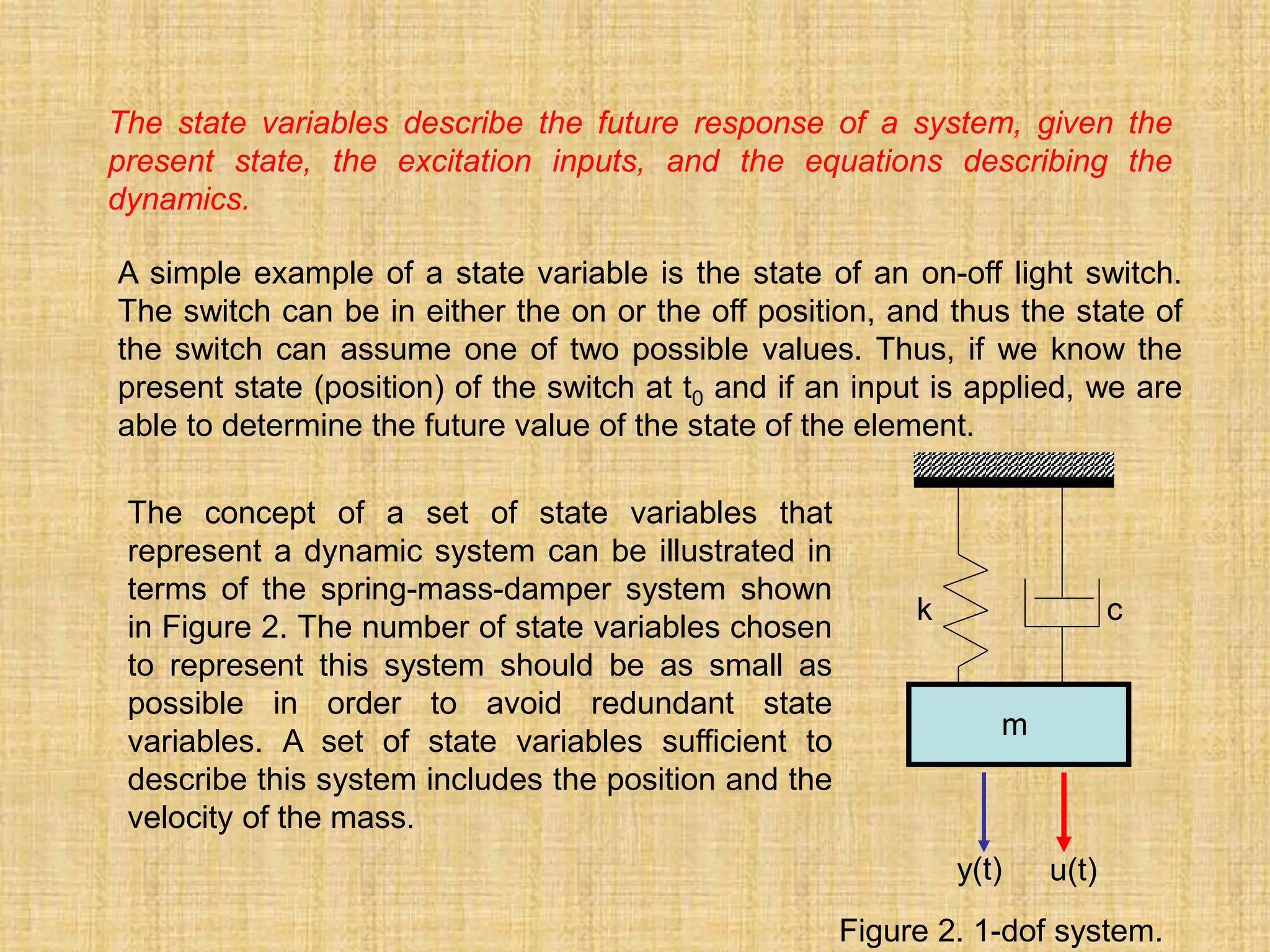
9. We can write the equations as a set of two first order differential equations in
terms of the state variables x1 [vC(t)] and x2 [iL(t)] as follows:
2
1
2
2
1
x
L
R
x
L
1
dt
dx
)
t
(
u
C
1
x
C
1
dt
dx





L
c
i
)
t
(
u
dt
dv
C 

c
L
L
v
i
R
dt
di
L 


The output signal is then 2
0
1 x
R
)
t
(
v
)
t
(
y 

Utilizing the first-order differential equations and the initial conditions of the
network represented by [x1(t0) x2(t0)], we can determine the system’s future
and its output.
The state variables that describe a system are not a unique set, and several
alternative sets of state variables can be chosen. For the RLC circuit, we
might choose the set of state variables as the two voltages, vC(t) and vL(t).

10. In an actual system, there are several choices of a set of state variables that
specify the energy stored in a system and therefore adequately describe the
dynamics of the system.
The state variables of a system characterize the dynamic behavior of a
system. The engineer’s interest is primarily in physical, where the variables
are voltages, currents, velocities, positions, pressures, temperatures, and
similar physical variables.
The State Differential Equation:
The state of a system is described by the set of first-order differential
equations written in terms of the state variables [x1 x2 ... xn]. These first-
order differential equations can be written in general form as
m
nm
1
1
n
n
nn
2
2
n
1
1
n
n
m
m
2
1
21
n
n
2
2
22
1
21
2
m
m
1
1
11
n
n
1
2
12
1
11
1
u
b
u
b
x
a
x
a
x
a
x
u
b
u
b
x
a
x
a
x
a
x
u
b
u
b
x
a
x
a
x
a
x


























11. Thus, this set of simultaneous differential equations can be written in matrix
form as follows:


























































m
1
nm
1
n
m
1
11
n
2
1
nn
2
n
1
n
n
2
22
21
n
1
12
11
n
2
1
u
u
b
b
b
b
x
x
x
a
a
a
a
a
a
a
a
a
x
x
x
dt
d















n: number of state variables, m: number of inputs.
The column matrix consisting of the state variables is called the state vector
and is written as













n
2
1
x
x
x
x

Dorf and Bishop, Modern Control Systems

12. The vector of input signals is defined as u. Then the system can be
represented by the compact notation of the state differential equation as
u
B
x
A
x 


This differential equation is also commonly called the state equation. The
matrix A is an nxn square matrix, and B is an nxm matrix. The state differential
equation relates the rate of change of the state of the system to the state of the
system and the input signals. In general, the outputs of a linear system can be
related to the state variables and the input signals by the output equation
u
D
x
C
y 

Where y is the set of output signals expressed in column vector form. The
state-space representation (or state-variable representation) is comprised of
the state variable differential equation and the output equation.

13. )
t
(
u
0
C
1
x
L
R
L
1
C
1
0
x























We can write the state variable differential equation for the RLC circuit as
and the output as
 x
R
0
y 
The solution of the state differential equation can be obtained in a manner
similar to the approach we utilize for solving a first order differential equation.
Consider the first-order differential equation
bu
ax
x 


Where x(t) and u(t) are scalar functions of time. We expect an exponential
solution of the form eat. Taking the Laplace transform of both sides, we have

14. )
s
(
U
b
)
s
(
X
a
x
)
s
(
X
s 0 


therefore,
)
s
(
U
a
s
b
a
s
)
0
(
x
)
s
(
X




The inverse Laplace transform of X(s) results in the solution
 


 

t
0
)
t
(
a
at
d
)
(
u
b
e
)
0
(
x
e
)
t
(
x
We expect the solution of the state differential equation to be similar to x(t)
and to be of differential form. The matrix exponential function is defined
as

 





!
k
t
A
!
2
t
A
At
I
e
k
k
2
2
At
Dorf and Bishop, Modern Control Systems

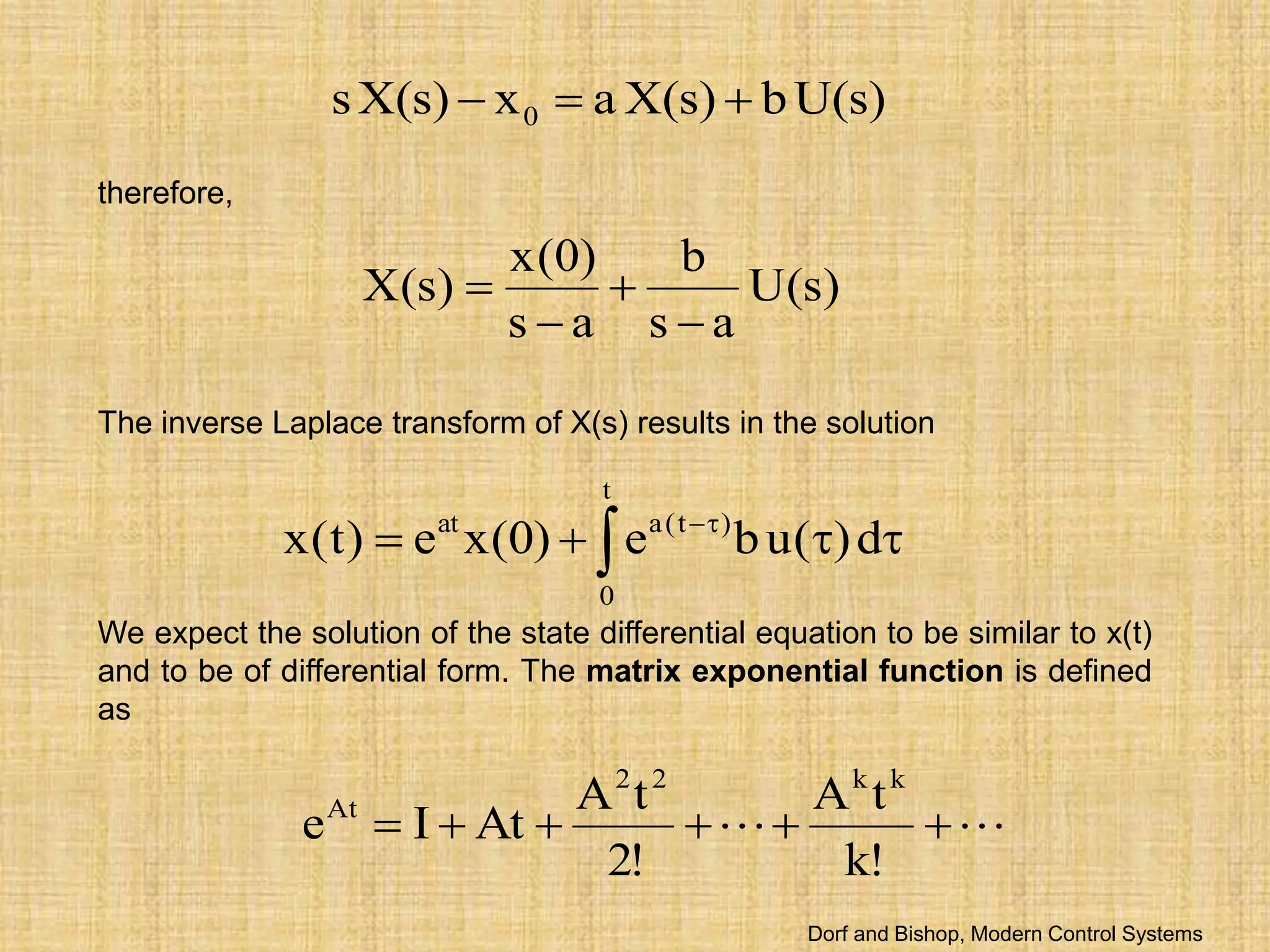
15. which converges for all finite t and any A. Then the solution of the state
differential equation is found to be
    )
s
(
U
B
A
sI
)
0
(
x
A
sI
)
s
(
X
d
)
(
u
B
e
)
0
(
x
e
)
t
(
x
1
1
t
0
)
t
(
A
At











 
where we note that [sI-A]-1=ϕ(s), which is the Laplace transform of ϕ(t)=eAt.
The matrix exponential function ϕ(t) describes the unforced response of
the system and is called the fundamental or state transition matrix.
 







t
0
d
)
(
u
B
)
t
(
)
0
(
x
)
t
(
)
t
(
x
Dorf and Bishop, Modern Control Systems

16. THE TRANSFER FUNCTION FROM THE STATE EQUATION
The transfer function of a single input-single output (SISO) system can be
obtained from the state variable equations.
u
B
x
A
x 


x
C
y 
where y is the single output and u is the single input. The Laplace transform
of the equations
)
s
(
CX
)
s
(
Y
)
s
(
U
B
)
s
(
AX
)
s
(
sX



where B is an nx1 matrix, since u is a single input. We do not include initial
conditions, since we seek the transfer function. Reordering the equation

17.  
)
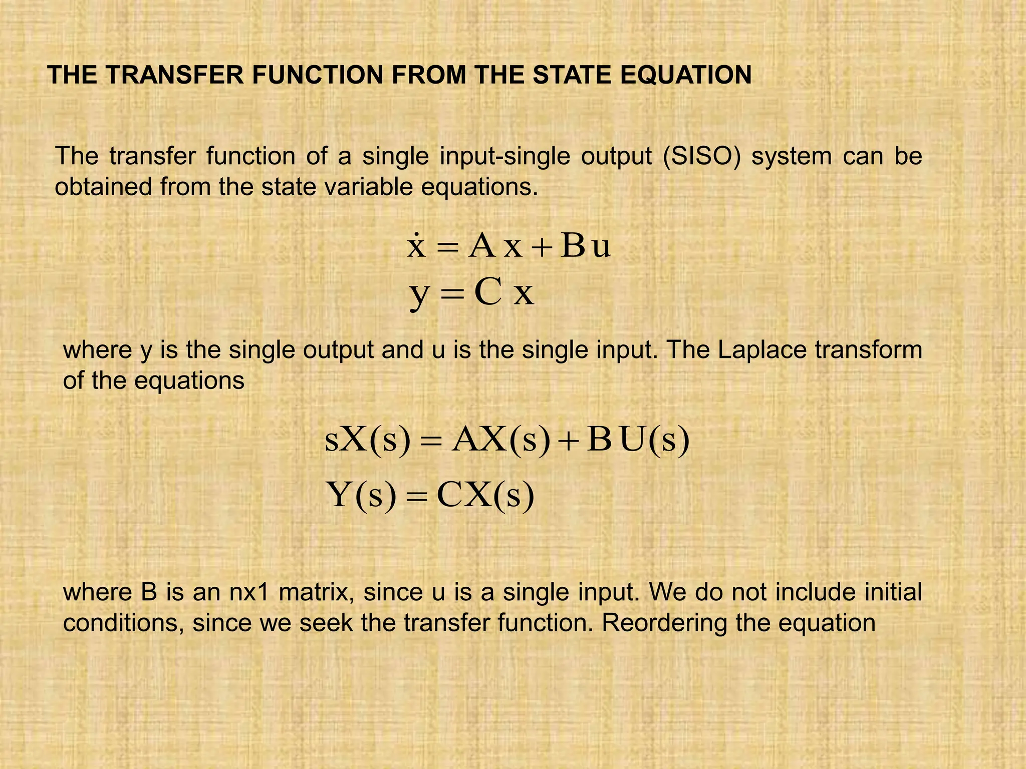
s
(
BU
)
s
(
C
)
s
(
Y
)
s
(
BU
)
s
(
)
s
(
BU
A
sI
)
s
(
X
)
s
(
U
B
)
s
(
X
]
A
sI
[
1









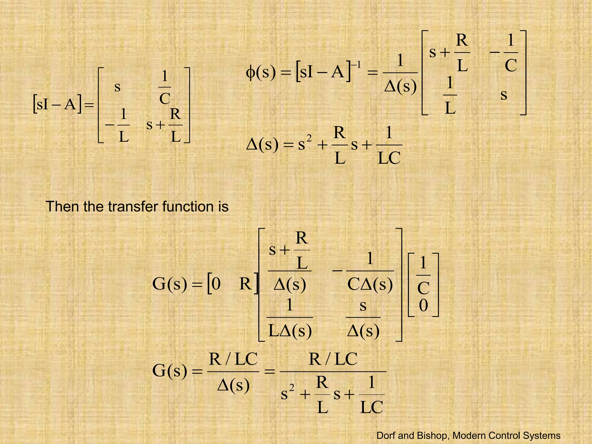
Therefore, the transfer function G(s)=Y(s)/U(s) is
B
)
s
(
C
)
s
(
G 

Example:
Determine the transfer function G(s)=Y(s)/U(s) for the RLC circuit as described
by the state differential function
 x
R
0
y
,
u
0
C
1
x
L
R
L
1
C
1
0
x 
























18.  














L
R
s
L
1
C
1
s
A
sI
 
LC
1
s
L
R
s
)
s
(
s
L
1
C
1
L
R
s
)
s
(
1
A
sI
)
s
(
2
1






















Then the transfer function is
 
LC
1
s
L
R
s
LC
/
R
)
s
(
LC
/
R
)
s
(
G
0
C
1
)
s
(
s
)
s
(
L
1
)
s
(
C
1
)
s
(
L
R
s
R
0
)
s
(
G
2


































Dorf and Bishop, Modern Control Systems

19. ANALYSIS OF STATE VARIABLE MODELS USING MATLAB
Given a transfer function, we can obtain an equivalent state-space representation
and vice versa. The function tf can be used to convert a state-space
representation to a transfer function representation; the function ss can be used
to convert a transfer function representation to a state-space representation. The
functions are shown in Figure 4, where sys_tf represents a transfer function model
and sys_ss is a state space representation.
Linear system model conversion
State-space object
Du
Cx
y
Bu
Ax
x





sys=ss(A,B,C,D)
Du
Cx
y
Bu
Ax
x




 )
s
(
U
)
s
(
G
)
s
(
Y 
sys_ss=ss(sys_tf)
sys_tf=tf(sys_ss)
)
s
(
U
)
s
(
G
)
s
(
Y 
Du
Cx
y
Bu
Ax
x





Figure 4.
The ss function
Dorf and Bishop, Modern Control Systems

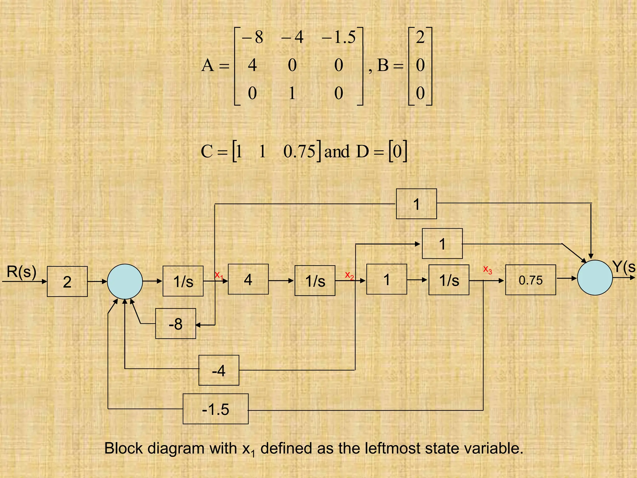
20. For instance, consider the third-order system
6
s
16
s
8
s
6
s
8
s
2
)
s
(
R
)
s
(
Y
)
s
(
G 2
3
2







We can obtain a state-space representation using the ss function. The state-
space representation of the system given by G(s) is
num=[2 8 6];den=[1 8 16 6];
sys_tf=tf(num,den)
sys_ss=ss(sys_tf)
Matlab code Transfer function:
2 s^2 + 8 s + 6
----------------------
s^3 + 8 s^2 + 16 s + 6
a =
x1 x2 x3
x1 -8 -4 -1.5
x2 4 0 0
x3 0 1 0
b =
u1
x1 2
x2 0
x3 0
c =
x1 x2 x3
y1 1 1 0.75
d =
u1
y1 0
Continuous-time model.
Answer
   
0
D
and
75
.
0
1
1
C
0
0
2
B
,
0
1
0
0
0
4
5
.
1
4
8
A






















 




21. 2
R(s)
1/s
-8
4
x1
1/s 1 1/s
x3 Y(s)
1
-4
-1.5
2
R(s)
-8
1/s
x2
1/s 0.75
1
1
Block diagram with x1 defined as the leftmost state variable.
   
0
D
and
75
.
0
1
1
C
0
0
2
B
,
0
1
0
0
0
4
5
.
1
4
8
A






















 




22. We can use the function expm to compute the transition matrix for a given
time. The expm(A) function computes the matrix exponential. By contrast the
exp(A) function calculates ea
ij for each of the elements aijϵA.
 


 

t
0
)
t
(
A
At
d
)
(
u
B
e
)
0
(
x
e
)
t
(
x
 







t
0
d
)
(
u
B
)
t
(
)
0
(
x
)
t
(
)
t
(
x
For the RLC network, the state-space representation is given as:
   
0
D
and
0
1
C
,
0
2
B
,
3
1
2
0
A 

















The initial conditions are x1(0)=x2(0)=1 and the input u(t)=0. At t=0.2, the state
transition matrix is calculated as
>>A=[0 -2;1 -3], dt=0.2; Phi=expm(A*dt)
Phi =
0.9671 -0.2968
0.1484 0.5219

23. The state at t=0.2 is predicted by the state transition method to be


















 









6703
.
0
6703
.
0
x
x
5219
.
0
1484
.
0
2968
.
0
9671
.
0
x
x
0
t
2
1
2
.
0
t
2
1
The time response of a system can also be obtained by using lsim
function. The lsim function can accept as input nonzero initial conditions
as well as an input function. Using lsim function, we can calculate the
response for the RLC network as shown below.
t
u(t)
Du
Cx
y
Bu
Ax
x





System
Arbitrary Input Output
t
y(t)
y(t)=output response at t
T: time vector
X(t)=state response at t
t=times at which
response is
computed
Initial conditions
(optional)
u=input
[y,T,x]=lsim(sys,u,t,x0)
Dorf and Bishop, Modern Control Systems

24. clc;clear
A=[0 -2;1 -3];B=[2;0];C=[1 0];D=[0];
sys=ss(A,B,C,D) %state-space model
x0=[1 1]; %initial conditions
t=[0:0.01:1];
u=0*t; %zero input
[y,T,x]=lsim(sys,u,t,x0);
subplot(211),plot(T,x(:,1))
xlabel('Time (seconds)'),ylabel('X_1')
subplot(212),plot(T,x(:,2))
xlabel('Time (seconds)'),ylabel('X_2')
0 0.2 0.4 0.6 0.8 1
0
0.2
0.4
0.6
0.8
1
Time (seconds)
X
1
0 0.2 0.4 0.6 0.8 1
0
0.2
0.4
0.6
0.8
1
Time (seconds)
X
2
Matlab code
0 0.1 0.2 0.3 0.4 0.5 0.6 0.7 0.8 0.9 1
0
1
2
3
Time (seconds)
X
1
0 0.1 0.2 0.3 0.4 0.5 0.6 0.7 0.8 0.9 1
0.4
0.6
0.8
1
Time (seconds)
X
2
u=3*t
u=0*t
0 0.1 0.2 0.3 0.4 0.5 0.6 0.7 0.8 0.9 1
1
1.5
2
2.5
Time (seconds)
X
1
0 0.1 0.2 0.3 0.4 0.5 0.6 0.7 0.8 0.9 1
0.7
0.8
0.9
1
Time (seconds)
X
2
u=3*exp(-2*t)

25. Example: Dorf and Bishop, Modern Control Systems, p173.
Consider the head mount of a disk reader shown in
the figure. We will attempt to derive a model for the
system shown in Figure 5a. Here we identify the
motor mass M1 and the head mount mass as M2.
The flexure spring is represented by the spring
constant k. The force u(t) to drive the mass M1 is
generated by the DC motor. If the spring is
absolutely rigid (nonspringy), then we obtain the
simplifed model shown in Figure 5b. Typical
parameters for the two-mass system are given in
Table 1.
M1 M2
q(t) y(t)
u(t)
Force
Motor
mass
Head
mass
Head
position
b1
b2
M=M1+M2
y(t)
u(t)
b1
Figure 5a Figure 5b
Table 1. Typical parameters of the two-mass model
Motor mass M1= 0.02 kg Friction at mass 1 b1=410x10-3 kgs/m Motor constant Km=0.1025 Nm/A
Flexure spring 10<=k<=inf Field resistance R=1 Ω Friction at mass 2 b2=4.1x10-3 kgm/s
Head mounting M2=0.0005 kg Field inductance L=1 mH Head position y(t)=x2(t)

26.  
  0
q
y
k
dt
dy
b
dt
y
d
M
)
t
(
u
y
q
k
dt
dq
b
dt
q
d
M
2
2
2
2
1
2
2
1








To develop a state variable model, we
choose the state variables as x1=q and
x2=y. Then we have















4
3
x
y
x
q
y
q
x


In matrix form,
dt
dy
x
and
dt
dq
x 4
3 

Bu
Ax
x 



















2
2
2
2
1
1
1
1
M
/
b
0
M
/
k
M
/
k
0
M
/
b
M
/
k
M
/
k
1
0
0
0
0
1
0
0
A













0
M
/
1
0
0
B
1
Note that the output is dy/dt=x4. Also, for L=0 or negligible inductance, then
u(t)=Kmv(t). For the typical parameters and k=10, we have
Motor coil
R
Ls
Km

V(s) U(s)
Force
Two-
mass
system
 x
1
0
0
0
y 

27. 





























2
.
8
0
20000
20000
0
5
.
20
500
500
1
0
0
0
0
1
0
0
A
,
0
50
0
0
B
0 0.5 1 1.5
0
0.5
1
1.5
2
2.5
3
Time (seconds)
ydot
(m/s)
clc;clear
k=10;
M1=0.02;M2=0.0005;
b1=410e-3;b2=4.1e-3;
t=0:0.001:1.5;
A=[0 0 1 0;0 0 0 1;-k/M1 k/M1 -
b1/M1 0;k/M2 -k/M2 0 -b2/M2];
B=[0;0;1/M1;0];C=[0 0 0 1];D=[0];
sys=ss(A,B,C,D)
y=step(sys,t);
plot(t,y);grid
xlabel('Time
(seconds)'),ylabel('ydot (m/s)')
Velocity of Mass 2 (Head)
Dorf and Bishop, Modern Control Systems
k=10 N/m

28. 0 0.5 1 1.5
0
0.5
1
1.5
2
2.5
Time (seconds)
ydot
(m/s)
k=100 N/m
0 0.5 1 1.5
0
0.5
1
1.5
2
2.5
Time (seconds)
ydot
(m/s)
k=1000 N/m
0 0.5 1 1.5
0
0.5
1
1.5
2
2.5
Time (seconds)
ydot
(m/s)
k=100000 N/m

29. THE DESIGN OF STATE VARIABLE FEEDBACK SYSTEMS
The time-domain method, expressed in terms of state variables, can also be utilized
to design a suitable compensation scheme for a control system. Typically, we are
interested in controlling the system with a control signal, u(t), which is a function of
several measurable state variables. Then we develop a state variable controller that
operates on the information available in measured form.
State variable design is typically comprised of three steps. In the first step, we
assume that all the state variables are measurable and utilize them in a full-state
feedback control law. Full-state feedback is not usually practical because it is not
possible (in general) to measure all the states. In paractice, only certain states (or
linear combinations thereof) are measured and provided as system outputs. The
second step in state varaible design is to construct an observer to estimate the
states that are not directly sensed and available as outputs. Observers can either
be full-state observers or reduced-order observers. Reduced-order observers
account for the fact that certain states are already available as system outputs;
hence they do not need to be estimated. The final step in the design process is to
appropriately connect the observer to the full-state feedback conrol low. It is
common to refer to the state-varaible controller as a compensator. Additionally, it is
possible to consider reference inputs to the state variable compensator to complete
the design.
Dorf and Bishop, Modern Control Systems

30. CONTROLLABILITY:
Full-state feedback design commonly relies on pole-placement
techniques. It is important to note that a system must be completely
controllable and completely observable to allow the flexibility to place all
the closed-loop system poles arbitrarily. The concepts of controllability and
observability were introduced by Kalman in the 1960s.
A system is completely controllable if there exists an unconstrained
control u(t) that can transfer any initial state x(t0) to any other desired
location x(t) in a finite time, t0≤t≤T.

31. For the system
Bu
Ax
x 


we can determine whether the system is controllable by examining the
algebraic condition
  n
B
A
B
A
AB
B
rank 1
n
2



The matrix A is an nxn matrix an B is an nx1 matrix. For multi input systems,
B can be nxm, where m is the number of inputs.
For a single-input, single-output system, the controllability matrix Pc is
described in terms of A and B as
 
B
A
B
A
AB
B
P 1
n
2
c

 
which is nxn matrix. Therefore, if the determinant of Pc is nonzero, the system
is controllable.

32. Example:
Consider the system
   u
0
x
0
0
1
y
,
u
1
0
0
x
a
a
a
1
0
0
0
1
0
x
2
1
0




























 

















































1
2
2
2
2
2
2
1
0 a
a
a
1
B
A
,
a
1
0
AB
,
1
0
0
B
,
a
a
a
1
0
0
0
1
0
A
 
 














1
2
2
2
2
2
c
a
a
a
1
a
1
0
1
0
0
B
A
AB
B
P
The determinant of Pc =1 and ≠0 , hence this system is controllable.

33. Example.
Consider a system represented by the two state equations
1
2
2
1
1 x
d
x
3
x
,
u
x
2
x 




 

The output of the system is y=x2. Determine the condition of controllability.
   u
0
x
1
0
y
,
u
0
1
x
3
d
0
2
x 























 






























d
0
2
1
P
d
2
0
1
3
d
0
2
AB
and
0
1
B
c The determinant of pc is equal to d, which is
nonzero only when d is nonzero.
Dorf and Bishop, Modern Control Systems

34. The controllability matrix Pc can be constructed in Matlab by using ctrb
command.






























2
.
8
0
20000
20000
0
5
.
20
500
500
1
0
0
0
0
1
0
0
A
,
0
50
0
0
B
From two-mass system,
Pc =
1.0e+007 *
0 0.0000 -0.0001 -0.0004
0 0 0 0.1000
0.0000 -0.0001 -0.0004 0.0594
0 0 0.1000 -2.8700
rank_Pc =
4
det_Pc =
-2.5000e+015
clc
clear
A=[0 0 1 0;0 0 0 1;-500 500 -20.5
0;20000 -20000 0 -8.2];
B=[0;0;50;0];
Pc=ctrb(A,B)
rank_Pc=rank(Pc)
det_Pc=det(Pc)
The system is
controllable.

35. OBSERVABILITY:
All the poles of the closed-loop system can be placed arbitrarily in the complex
plane if and only if the system is observable and controllable. Observability
refers to the ability to estimate a state variable.
A system is completely observable if and only if there exists a finite time T
such that the initial state x(0) can be determined from the
observation history y(t) given the control u(t).
Cx
y
and
Bu
Ax
x 



Consider the single-input, single-output system
where C is a 1xn row vector, and x is an nx1 column vector. This system is
completely observable when the determinant of the observability matrix P0
is nonzero.

36. The observability matrix, which is an nxn matrix, is written as













1
n
O
A
C
A
C
C
P

Example:
Consider the previously given system
 
0
0
1
C
,
a
a
a
1
0
0
0
1
0
A
2
1
0















Dorf and Bishop, Modern Control Systems

37.    
1
0
0
CA
,
0
1
0
CA 2


Thus, we obtain











1
0
0
0
1
0
0
0
1
PO
The det P0=1, and the system is completely observable. Note that
determination of observability does not utility the B and C matrices.
Example: Consider the system given by
 x
1
1
y
and
u
1
1
x
1
1
0
2
x 


















38. We can check the system controllability and observability using the Pc and P0
matrices.
From the system definition, we obtain
















2
2
AB
and
1
1
B
  









2
1
2
1
AB
B
Pc
Therefore, the controllability matrix is determined to be
det Pc=0 and rank(Pc)=1. Thus, the system is not controllable.
  









2
1
2
1
AB
B
Pc
Therefore, the controllability matrix is determined to be
Dorf and Bishop, Modern Control Systems

39. From the system definition, we obtain
   
1
1
CA
and
1
1
C 















1
1
1
1
CA
C
Po
Therefore, the observability matrix is determined to be
det PO=0 and rank(PO)=1. Thus, the system is not observable.
If we look again at the state model, we note that
2
1 x
x
y 

However,
  2
1
1
2
1
2
1 x
x
u
u
x
x
x
2
x
x 






 


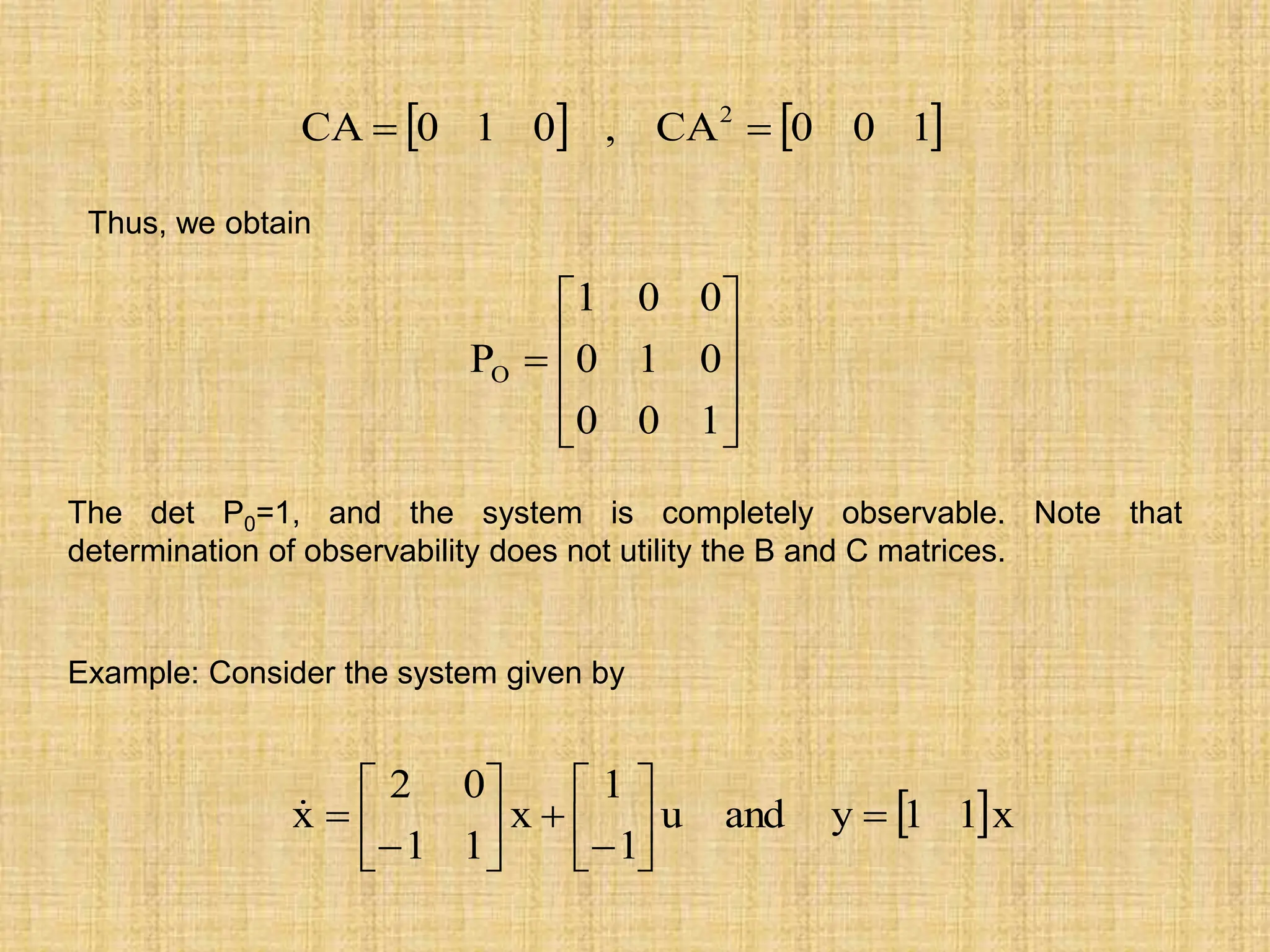
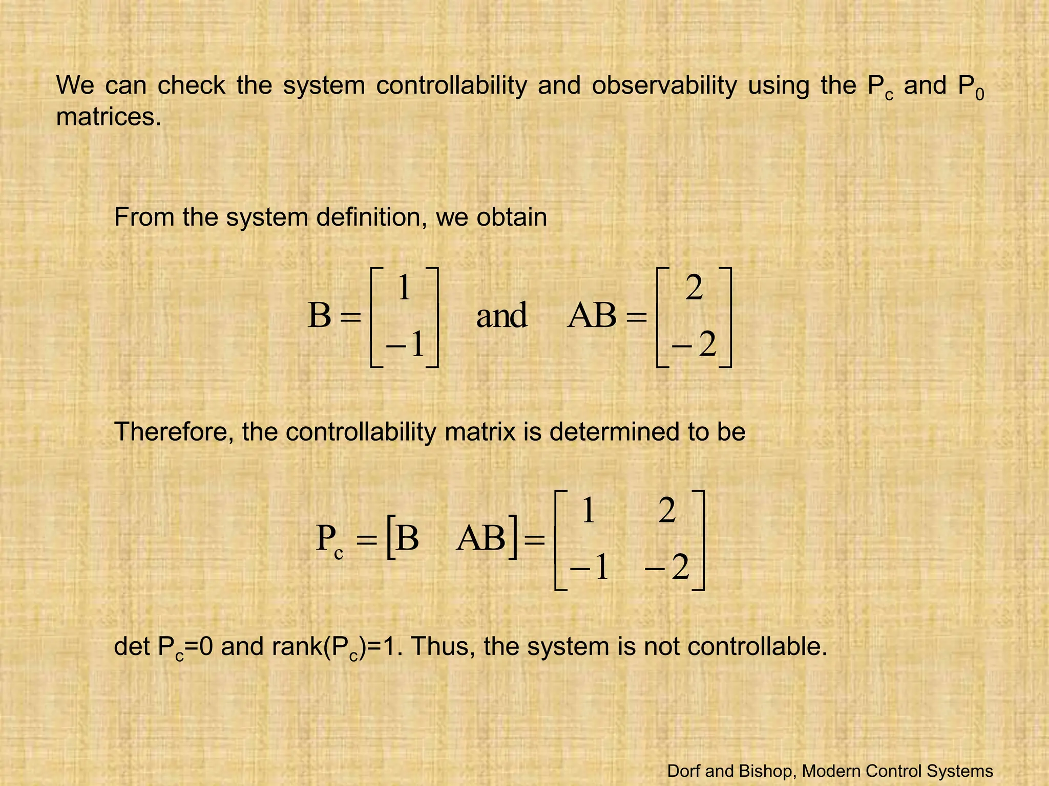
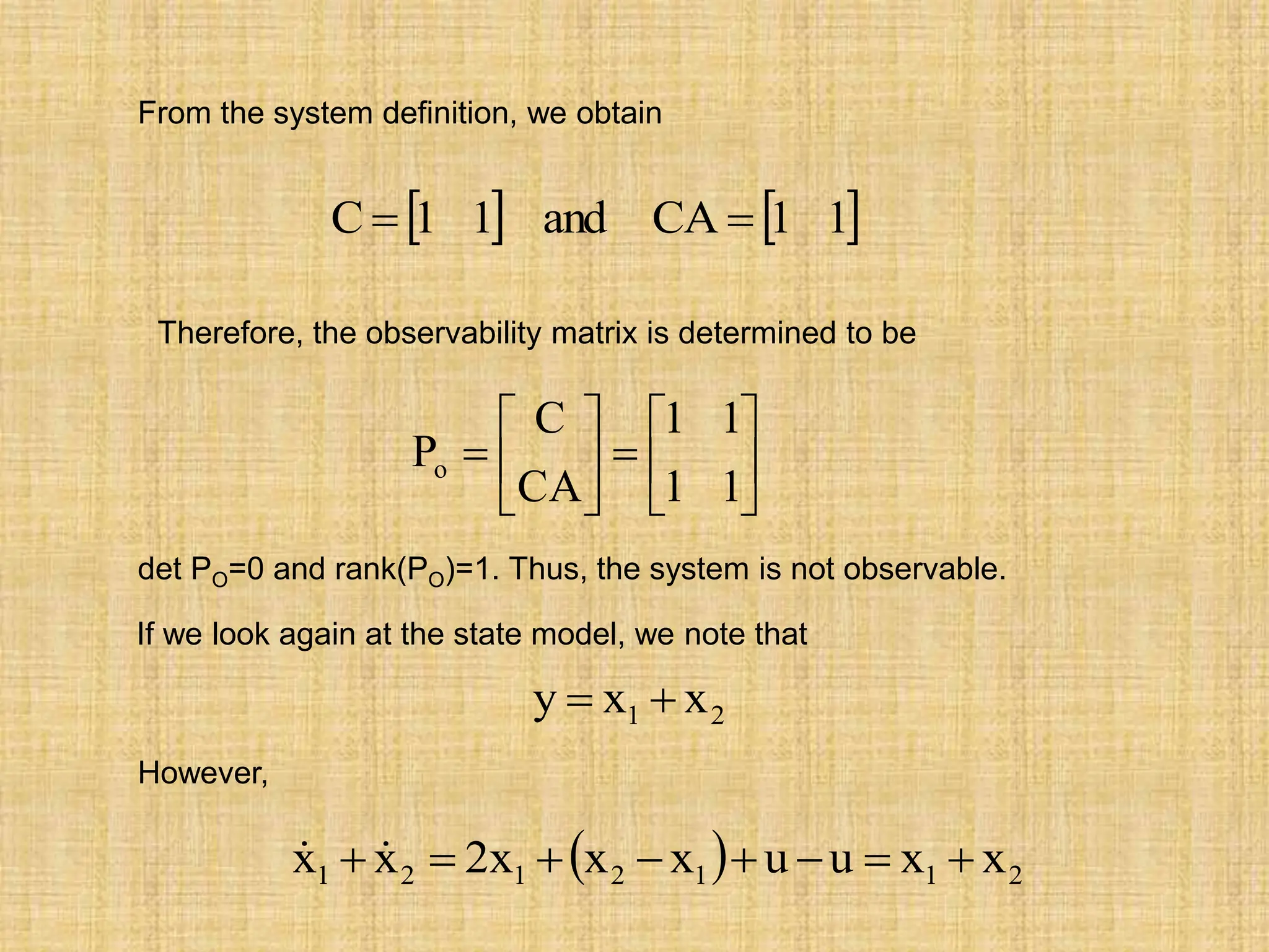
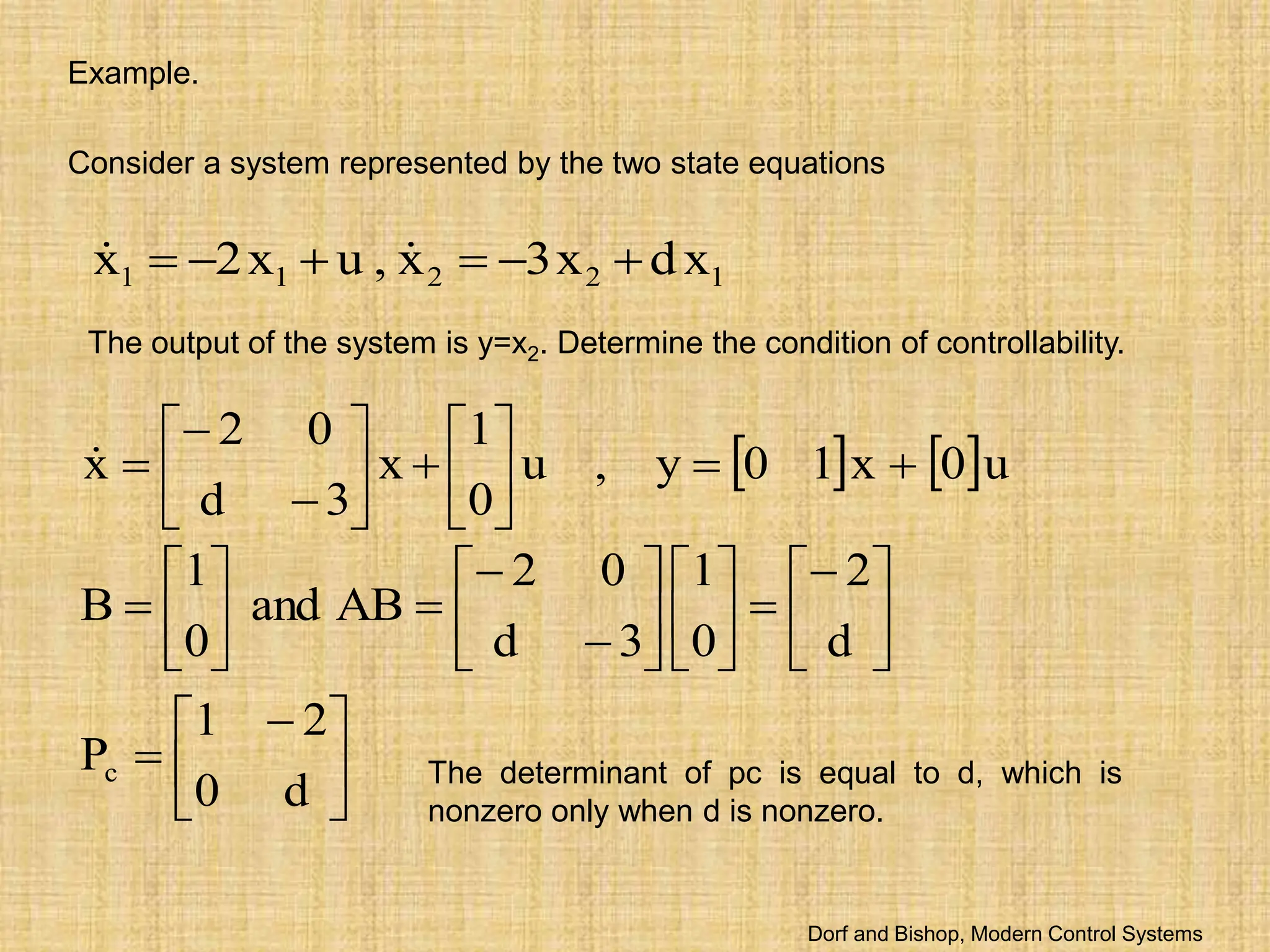
40. Thus, the system state variables do not depend on u, and the system is not
controllable. Similarly, the output (x1+x2) depends on x1(0) plus x2(0) and does
not allow us to determine x1(0) and x2(0) independently. Consequently, the
system is not observable.
The observability matrix PO can be constructed in Matlab by using obsv
command.
From two-mass system,
Po =
1 1
1 1
rank_Po =
1
det_Po =
0
clc
clear
A=[2 0;-1 1];
C=[1 1];
Po=obsv(A,C)
rank_Po=rank(Po)
det_Po=det(Po) The system is not
observable.
Dorf and Bishop, Modern Control Systems