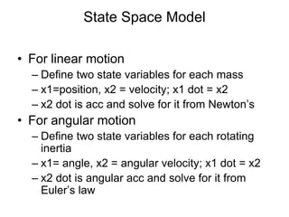
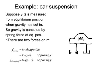
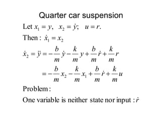
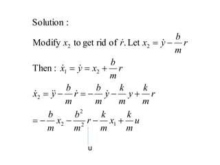
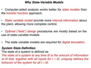
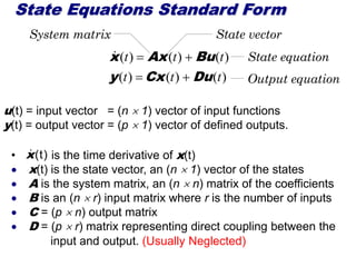
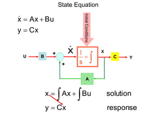
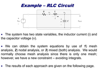
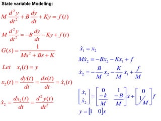
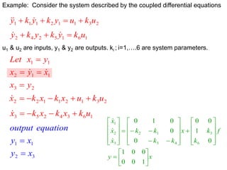
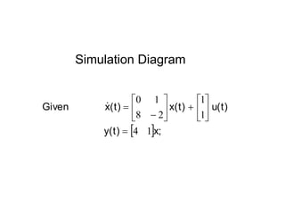
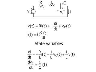
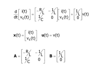
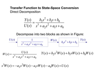
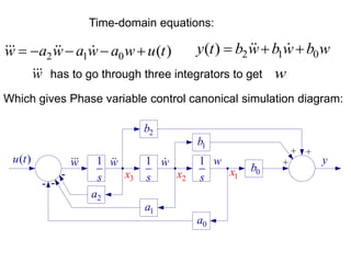
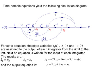
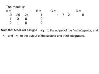
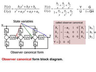
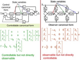
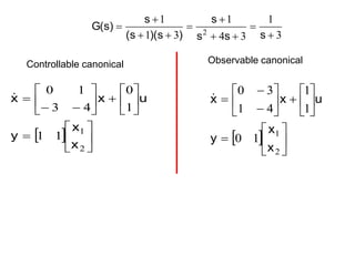
State variable models provide more internal information about a system compared to transfer function models, allowing for more complete control system design and analysis. The state of a system is defined as the minimum amount of information needed to uniquely determine the future behavior of the system given the inputs. State variable models are written in standard state space form with state, input, and output equations relating the state vector x, input vector u, and output vector y. An example RLC circuit is modeled using state space equations, and the solution is obtained using Laplace transforms.

1. Chapter 3
State Variable Models

2. Why State-Variable Models
• Computer-aided analysis works better for state models than
the transfer function approach.
• State variable model provide more internal information about
the plant, allowing more complete control.
• Optimal (“best”) design procedures are mostly based on the
use of state-variable models.
• The state variable models are required for digital simulation.
System State Definition
The state of a system is defined as
The state of a system at any time t0 is the amount of information
at t0 that, together with all inputs for t  t0, uniquely defines the
behavior of the system for all t  t0.

3. State Equations Standard Form
)
(
)
(
)
(
)
(
)
(
)
(
t
t
t
t
t
t
Du
Cx
y
Bu
Ax
x




 State equation
Output equation
State vector
System matrix
u(t) = input vector = (n  1) vector of input functions
y(t) = output vector = (p  1) vector of defined outputs.
• is the time derivative of x(t)
 x(t) is the state vector, an (n  1) vector of the states
 A is the system matrix, an (n  n) matrix of the coefficients
 B is an (n  r) input matrix where r is the number of inputs
 C = (p  n) output matrix
 D = (p  r) matrix representing direct coupling between the
input and output. (Usually Neglected)
)
t
(
x


4. Cx
y
Bu
Ax
x




B C
U
x

A
Y
X
+
+
response
Cx
y
solution
Bu
Ax
x


 

State Equation
Initial
Conditions

5. Example – RLC Circuit
 The system has two state variables, the inductor current (i) and
the capacitor voltage (v).
 We can obtain the system equations by use of 1) mesh
analysis, 2) nodal analysis, or 3) mixed (both) analysis. We would
normally choose mesh analysis since there is only one mesh;
however, we have a new constraint – avoiding integrals.
 The results of each approach are given on the following page.

6. System Equations








t
OUT
t
IN
idt
C
v
idt
C
dt
di
L
iR
v
Mixed
0
0
1
0
1
0
1
0
1
2
1
0
2
0
2
1
1









dt
dv
C
dt
)
v
v
(
L
dt
)
v
v
(
L
R
v
v
Analysis
Nodal
t
t
IN
0
0








dt
dv
C
i
v
dt
di
L
iR
v
Analysis
Mesh
IN
All three results are valid models but only the equations obtained
from the mixed analysis can be represented as state equations in
the standard form. The state equations are given below:
C
i
dt
dv
v
L
v
L
i
L
R
dt
di
IN





1
1
This form is frequently used in digital simulation.

7. State Equations
v
v
v
L
v
i
C
L
L
R
v
i
OUT
IN
C
C



































0
1
0
1
1


The state equations, in standard form, for the series RLC circuit
are:

8. Solution Using Transforms
)
866
.
0
5
.
0
)(
866
.
0
5
.
0
(
1
1
)
(
)
( 2
j
s
j
s
s
LC
s
L
R
s
LC
s
V
s
V
IN
OUT








The solution for vOUT(t) will have the form
t
j
t
j
OUT e
V
e
V
V
t
v )
866
.
0
5
.
0
(
2
)
866
.
0
5
.
0
(
1
0
)
( 






The constants V0, V1, and V2 are evaluated using partial fractions:
1
)
866
.
0
5
.
0
)(
866
.
0
5
.
0
(
1
0 



j
j
V
2887
.
0
5
.
0
)
732
.
1
)(
866
.
0
5
.
0
(
1
1 j
j
j
V 






2887
.
0
5
.
0
)
732
.
1
)(
866
.
0
5
.
0
(
1
2 j
j
j
V 



)
866
.
0
sin(
5774
.
0
)
866
.
0
cos(
1
)
( 5
.
0
5
.
0
t
e
t
e
t
v t
t
OUT





vOUT(t) can be obtained by taking the inverse:

9. IN
C
C
v
L
v
i
C
L
L
R
v
i


































0
1
0
1
1






































s
C
L
L
R
s
C
L
L
R
1
1
0
1
1
1
0
0
1
A
I
Formal Solution We may use the standard form directly:
The characteristic equation for a
set of state equations is given by
|I – A| where A is the system
matrix, I is the identity matrix,
and the  values are the
eigenvalues. The matrix |I – A|
is given by
Taking the determinant of this matrix yields 0
1
2








LC
L
R
A
I
This agrees with the previous results (the denominator of the
transform).

10. )
(
2
2
t
f
Ky
dt
dy
B
dt
y
d
M 


)
(
2
2
t
f
Ky
dt
dy
B
dt
y
d
M 



K
Bs
Ms
s
G


 2
1
)
(
y
t
x
Let 
)
(
1
)
(
)
(
)
(
)
( 1
2 t
x
dt
t
dx
dt
t
dy
t
x 



2
2
2
2
)
(
)
(
dt
t
y
d
dt
t
dx
x 


2
1 x
x 

f
Kx
Bx
x
M 


 1
2
2

M
f
x
M
K
x
M
B
x 


 1
2
2

 x
y
f
M
x
M
B
M
k
x
x
0
1
1
0
1
0
2
1





























State variable Modeling:

11. 2
3
1
1
2
1
1
1 u
k
u
y
k
y
k
y 


 


1
6
1
5
2
4
2 u
k
y
k
y
k
y 

 

Example: Consider the system described by the coupled differential equations
u1 & u2 are inputs, y1 & y2 are outputs. ki ; i=1,….6 are system parameters.
2
3
1
1
2
1
1
y
x
x
y
x
y
x
Let






2
3
1
2
1
1
2
2 u
k
u
x
k
x
k
x 





1
6
3
4
2
5
3 u
k
x
k
x
k
x 




3
2
1
1
x
y
x
y
equation
output


x
y
f
k
k
x
k
k
k
k
x
x
x











































1
0
0
0
0
1
0
1
0
0
0
0
0
1
0
6
3
4
5
1
2
3
2
1




12. Simulation Diagram
  ;
x
)
t
(
y
)
t
(
u
)
t
(
x
)
t
(
x
Given
1
4
1
1
2
8
1
0


















13. Control canonical (Controllable)
&
Observer Canonical (Observable)
Matrix A,B & C are constructed from the transfer
function.
Next - Examples

17. Next slides consider general standard Transfer Function

18. 2
2 1 0
3 2
2 1 0
( )
( )
Y s b s b s b
U s s a s a s a
 

  
2 1 0
2 3
2 1 0
2 3
( )
( ) 1
b b b
Y s s s s
a a a
U s
s s s
 

  
Dividing each term by the highest order of s yields
Control canonical form block diagram.
   
1 1
2 2
3 0 1 2 3
1
0 1 2 2
3
0 1 0 0
0 0 1 0
1
0
x x
x x u
x a a a x
x
y b b b x u
x
       
       
 
       
  
       
       
 
 
 
 
 
 
GH
G
U
Y



1
is canonical form

19. Transfer Function to State-Space Conversion
Direct Decomposition
2
2 1 0
3 2
2 1 0
( )
( )
b s b s b
Y s
U s s a s a s a
 

  
Decompose into two blocks as shown in Figure:
( )
W s
3 2
2 1 0
1
s a s a s a
  
2
2 1 0
b s b s b
 
( )
U s ( )
Y s
3 2
2 1 0
( )
( )
U s
W s
s a s a s a

  
2
2 1 0
( ) ( ) ( ) ( )
Y s b s W s b sW s b W s
  
3 2
2 1 0
( ) ( ) ( ) ( ) ( )
s W s a s W s a sW s a W s U s
    

20. Time-domain equations:
2 1 0 ( )
w a w a w a w u t
     2 1 0
( )
y t b w b w b w
  
w has to go through three integrators to get w
Which gives Phase variable control canonical simulation diagram:
2
x
w 1
s
1
s
1
s 1
x
3
x
y
( )
u t
- -
-
w w w
0
a
1
a
2
a
0
b
2
b
1
b
+
+
+

21. 1
s 1
s
1
s
( )
u t
1
y
1
x
2
x
3
x
w w w w
0
a

1
a

2
a

0
b
1
b
2
b
1
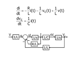
Signal flow graph similar to the Simulation diagram :
Control System Toolbox contains a set of functions for model
conversion:
G = tf(num, den)
[A, B, C, D] = tf2ss(num, den), [num, den] = ss2tf(A, B, C, D, 1)
Converts the system in transfer function form to state-space phase
variable control canonical form & vice versa
For list of all functions type help/control/control at MATLAB prompt

22. Example:
For the following transfer function:
2
3 2
( ) 7 2
( )
( ) 9 26 24
Y s s s
G s
U s s s s
 
 
  
(a) Draw the simulation diagram and find the state-space
representation of the above transfer function.
(b) Use MATLAB Control System Toolbox
[A, B, C, D] = tf2ss(num, den) to find the state model.
Sol: a) Draw the transfer function block diagram in cascade form
3 2
1
9 26 24
s s s
  
2
7 2
s s
 
( )
Y s
( )
U s ( )
W s
From this we have:
3 2 2
( ) 9 ( ) 26 ( ) 24 ( ) ( ) & ( ) ( ) 7 ( ) 2 ( )
s W s s W s sW s W s U s Y s s W s sW s W s
       
or in time-domain 9 26 24 & y 7 2
w w w w u w w w
       

23. Time-domain equations yield the following simulation diagram:
1
s 1
s
1
s
( )
u t
1
y
1
x
2
x
3
x
w w w w
24

26

9

2
7
1
1
For state equation, the state variables , and
1( )
x t 2 ( )
x t 3( )
x t
are assigned to the output of each integrator from the right to the
left. Next an equation is written for the input of each integrator.
The results are:
1 2
x x
 2 3
x x
 3 1 2 1
24 26 9 ( )
x x x x u t
    
and the output equation is: 1 2 3
2 7
y x x x
  

24. Hence, in matrix form
1 1
2 2
3 3
0 1 0 0
0 0 1 0 ( )
24 26 9 1
x x
x x u t
x x
   
   
   
   
 
   
   
   
   
  
   
   
 
1
2
3
2 7 1
x
y x
x
 
 
  
 
 
(b) Re-write the following statements:
num = [1 7 2]; den = [1 9 26 24];
[A, B, C, D] = tf2ss(num, den)

25. The result is:
A = B = C = D =
-9 -26 -24 1 1 7 2 0
1 0 0 0
0 1 0 0
Note that MATLAB assigns 1
x to the output of the first integrator, and
2
x and 3
x to the output of the second and third integrators.

26. 2 1 0
2 2 3 2 3
3 2
2 1 0
2 3 2 3
2 8 6
( ) 2 8 6
8 26 6
( ) 8 26 6 1 1
b b b
C s s s s s s s s s
a a a
R s s s s
s s s s s s
   
 
  
        
The form is:
 
1 1
2 2
3 3
1
2
3
0 1 0 0
0 0 1 0
6 26 8 1
6 8 2 [0] .
x x
x x r
x x
x
y x r
x
       
       
 
       
  
       
       
 
 
 
 
 
 
System controllable but not observable. Why?
Ans: State model is based on controllable canonical form, this
can be confirmed by another method later.
is controllable canonical form
Example:

27. Observer canonical form block diagram.
2
2 1 0
3 2
2 1 0
( )
( )
Y s b s b s b
U s s a s a s a
 

  
2 1 0
2 3
2 1 0
2 3
( )
( ) 1
b b b
Y s s s s
a a a
U s
s s s
 

   GH
G
U
Y



1
 
0
0
1
0
0
1
0
0
1
2
1
0
3
2
1
0
1
2
3
2
1














































Y
u
b
b
b
X
X
X
a
a
a
X
X
X



called observer canonical

28.  
























































3
2
1
2
1
0
3
2
1
0
1
2
3
2
1
0
0
1
0
0
1
0
0
1
X
X
X
Y
u
b
b
b
X
X
X
a
a
a
X
X
X



  













































3
2
1
2
1
0
1
0
0
3
2
1
2
1
0
1
0
0
0
1
0
3
2
1
X
X
X
b
b
b
Y
u
X
X
X
a
a
a
X
X
X



observable but not directly
controllable
Controllable but not directly
observable
Controllable canonical form

29. 3
1
3
4
1
3
1
1
2 









s
s
s
s
)
s
)(
s
(
s
)
s
(
G
Controllable canonical
  






















2
1
1
1
1
0
4
3
1
0
x
x
y
u
x
x

Observable canonical
  






















2
1
1
0
1
1
4
1
3
0
x
x
y
u
x
x


30. Modeling
• Types of systems electric
mechanical
electromechanical
• Types of models I/O o.d.e. models
Transfer Function
state space models



31. I/O o.d.e. model: o.d.e. involving input/output only.
linear:
where u: input
y: output
u
b
u
dt
d
b
u
dt
d
b
y
a
y
dt
d
a
y
dt
d
a
y
dt
d
m
m
m
n
n
n
n
n
0
1
0
1
1
1
1







 





32. State space model:
linear:
or in some text:
where: u: input
y: output
x: state vector
A,B,C,D, or F,G,H,J are constt matrices





)
,
(
:
eq
Output
)
,
(
:
eq
State
u
x
h
y
u
x
f
x








Du
Cx
y
Bu
Ax
x








Ju
Hx
y
Gu
Fx
x


33. Other types of models:
Transfer function model (This is I/O model)
from I/O o.d.e. model, take Laplace
transform:
  ),
(
)
( s
Y
t
y 
L
)
(
)
( s
sY
t
y
dt
d







L

),
(
)
( 2
2
2
s
Y
s
t
y
dt
d







L
  ),
(
)
( s
U
t
u 
L )
(
)
( s
sU
t
u
dt
d







L

34. Then I/O model in L.T. domain becomes:
This is the T.F. model of the system.
∴T.F.
or
i.e. output L.T. is eq. to input L.T. with gain H(s)
)
(
)
(
)
(
)
(
)
(
)
(
)
(
0
1
0
1
1
1
s
U
b
s
sU
b
s
U
s
b
s
Y
a
s
sY
a
s
Y
s
a
s
Y
s
m
m
n
n
n







 



0
1
1
1
0
1
)
(
)
(
a
s
a
s
a
s
b
s
b
s
b
s
U
s
Y
n
n
n
m
m







 
 

denote
 )
(
or
)
( s
G
s
H
)
(
)
(
)
(
or
)
(
s
U
s
Y
s
G
s
H 
)
(
)
(
or
)
(
)
(
)
( s
U
s
G
s
U
s
H
s
Y 

35. State space model to T.F. / block diagram:
s.s.
Take L.T. :
From sX(s)-AX(s)=BU(s)
sIX(s)-AX(s)=BU(s)
(sI-A)X(s)=BU(s)
X(s)=(sI-A)-1BU(s)







Du
Cx
y
Bu
Ax
x








)
(
)
(
)
(
)
(
)
(
)
(
s
DU
s
CX
s
Y
s
BU
s
AX
s
sX 1
2
1

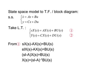
36. into : Y(s)=C(sI-A)-1BU(s)+DU(s)
Y(s)=[C(sI-A)-1B+D] U(s)
G(s)= D+C(sI-A)-1B
is the T.F. from u to y
from
))
(
)
(
(
1
)
( s
BU
s
AX
s
s
X 

2


 


 

1
1
s
u(s) +
+
x(s)
B C
A
+
+
D
y(s)

37. Example
 






















x
y
u
x
x
3
1
1
0
3
2
1
0

 


















1
0
,
3
2
1
0
3
1
,
0
B
A
C
D

38.  
 
 
 
 
2
3
1
3
2
)
3
(
1
3
1
3
1
2
)
3
(
1
1
2
)
3
(
1
3
1
1
0
2
1
3
2
)
3
(
1
3
1
1
0
3
2
1
3
1
1
0
3
2
1
0
1
0
0
1
3
1
0
)
(
)
(
2
1
1
1





























































































s
s
s
s
s
s
s
s
s
s
s
s
s
s
s
s
s
s
s
B
A
sI
C
D
s
G

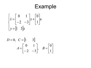
39. • In Matlab:
>> A=[0 1;-2 -3];
>> B=[0;1];
>> C=[1 3];
>> D=[0];
>> [n,d]=ss2tf(A,B,C,D)
n =
0 3.0000 1.0000
d =
1 3 2
>> n=[1 2 3];d=[1 4 5 6];
>> [A,B,C,D]=tf2ss(n,d)
A =
-4 -5 -6
1 0 0
0 1 0
B =
1
0
0
C =
1 2 3
D =
0
>> tf(n,d)
Transfer function:
s^2 + 2 s + 3
---------------------
s^3 + 4 s^2 + 5 s + 6

40. State Space Model
• For linear motion
– Define two state variables for each mass
– x1=position, x2 = velocity; x1 dot = x2
– x2 dot is acc and solve for it from Newton’s
• For angular motion
– Define two state variables for each rotating
inertia
– x1= angle, x2 = angular velocity; x1 dot = x2
– x2 dot is angular acc and solve for it from
Euler’s law

41. Example: car suspension
Suppose y(t) is measured
from equilibrium position
when gravity has set in.
So gravity is canceled by
spring force at eq. pos.
∴There are two forces on m:
y
)
r
y
(
b
f
y
(y-r)
k
elongation
k
f
damping
spring


 opposing
opposing








42. Quarter car suspension
r
u
m
k
r
m
b
x
m
k
x
m
b
r
m
k
r
m
b
y
m
k
y
m
b
y
x
x
x
r
u
y
x
y
x









:
input
nor
state
neither
is
variable
One
:
Problem
:
Then
.
;
,
Let
1
2
2
2
1
2
1
















43. u
m
k
x
m
k
r
m
b
x
m
b
r
m
k
y
m
k
y
m
b
r
m
b
y
x
r
m
b
x
y
x
r
m
b
y
x
r
x
















1
2
2
2
2
2
1
2
2
:
Then
Let
.
of
rid
get
to
Modify
:
Solution









u

44.    u
x
x
x
y
u
m
b
m
k
m
b
x
x
m
b
m
k
x
x
0
0
1
1
0
:
form
matrix
in
model
space
State
2
1
1
2
2
2
1
2
1





















































