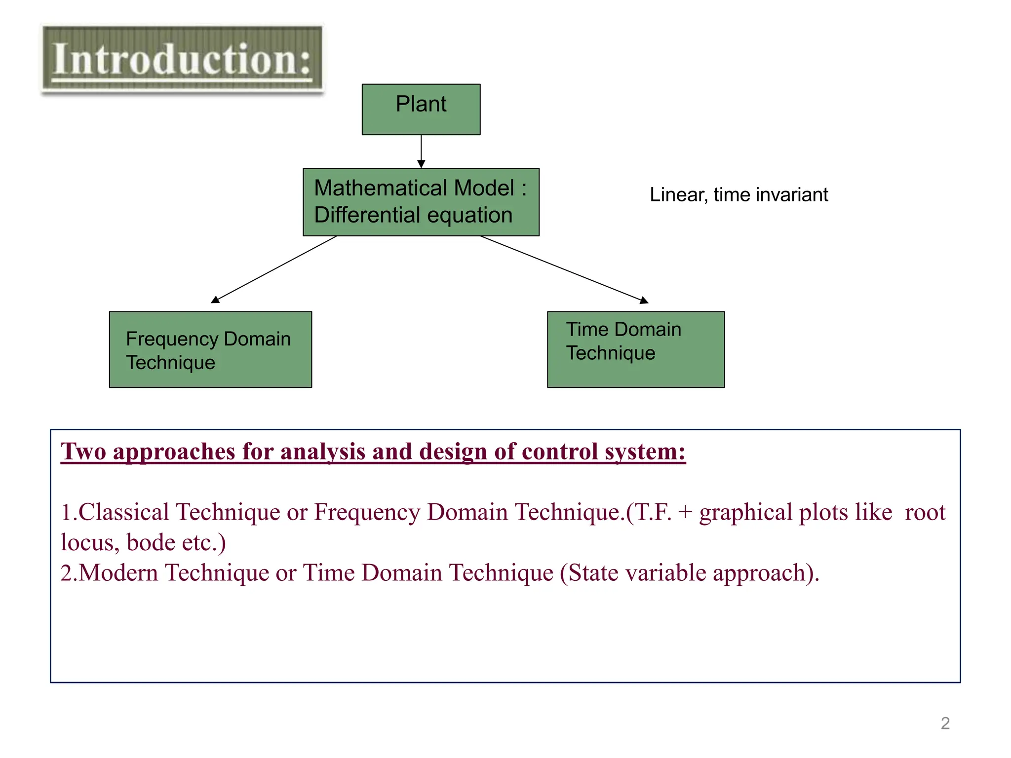
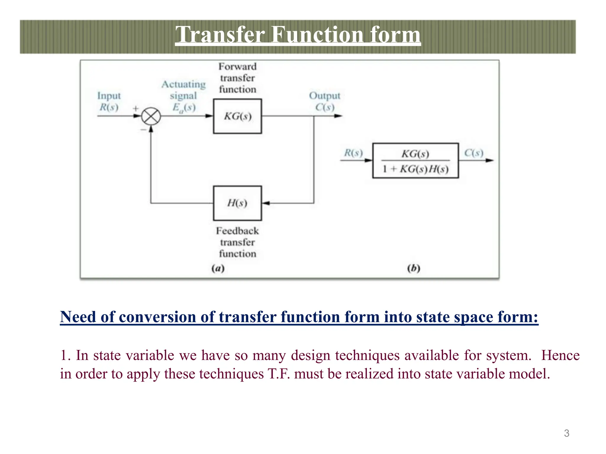
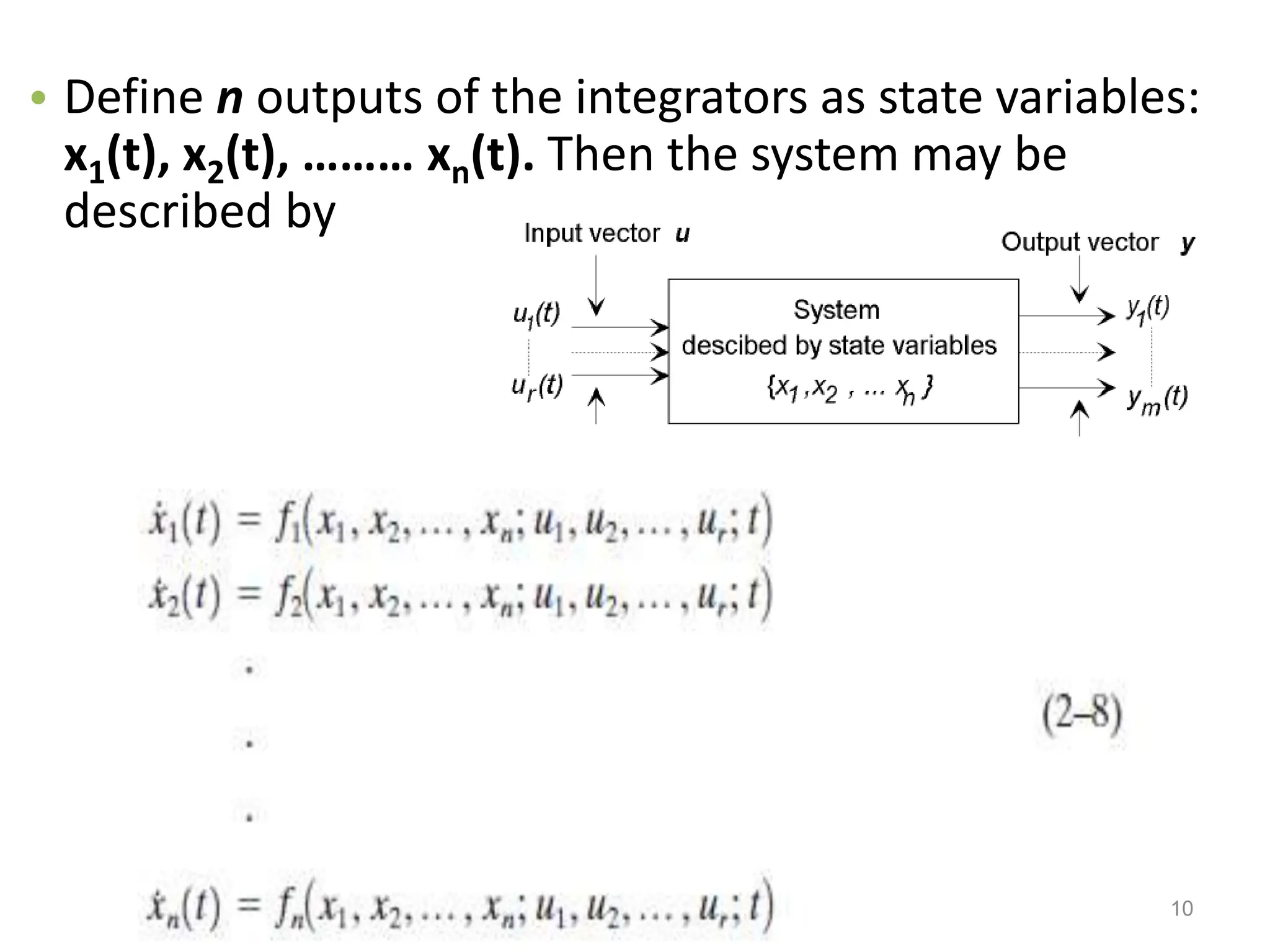
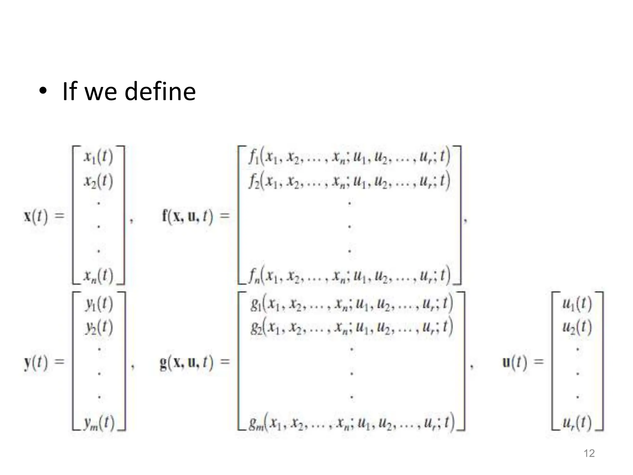
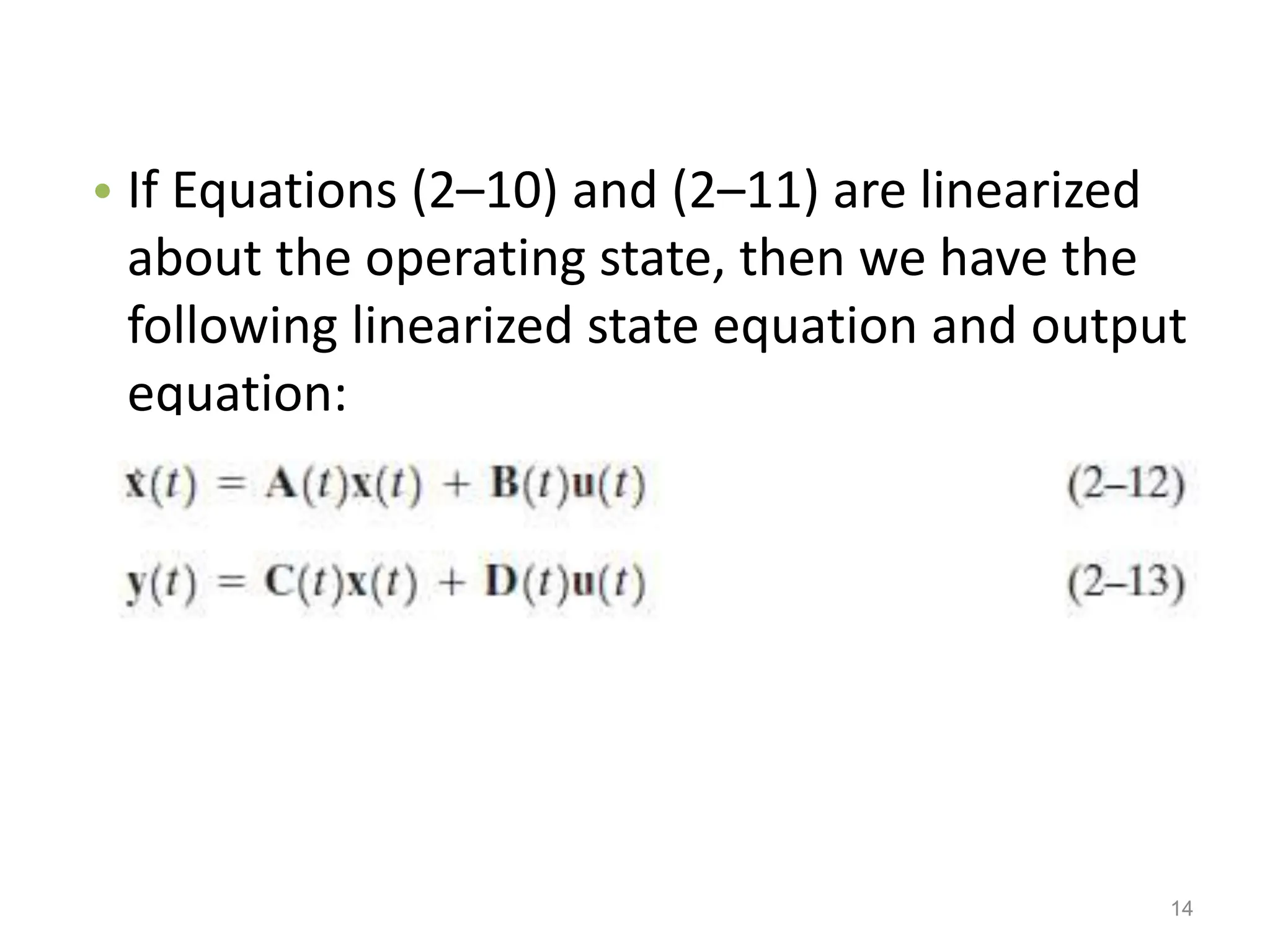
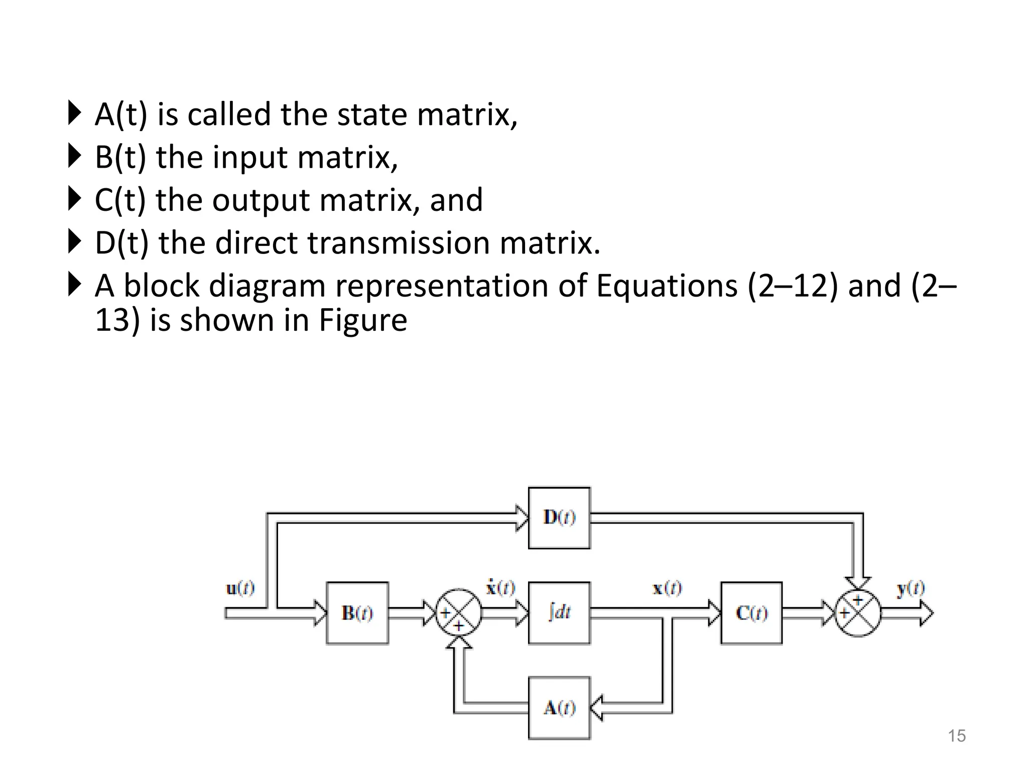
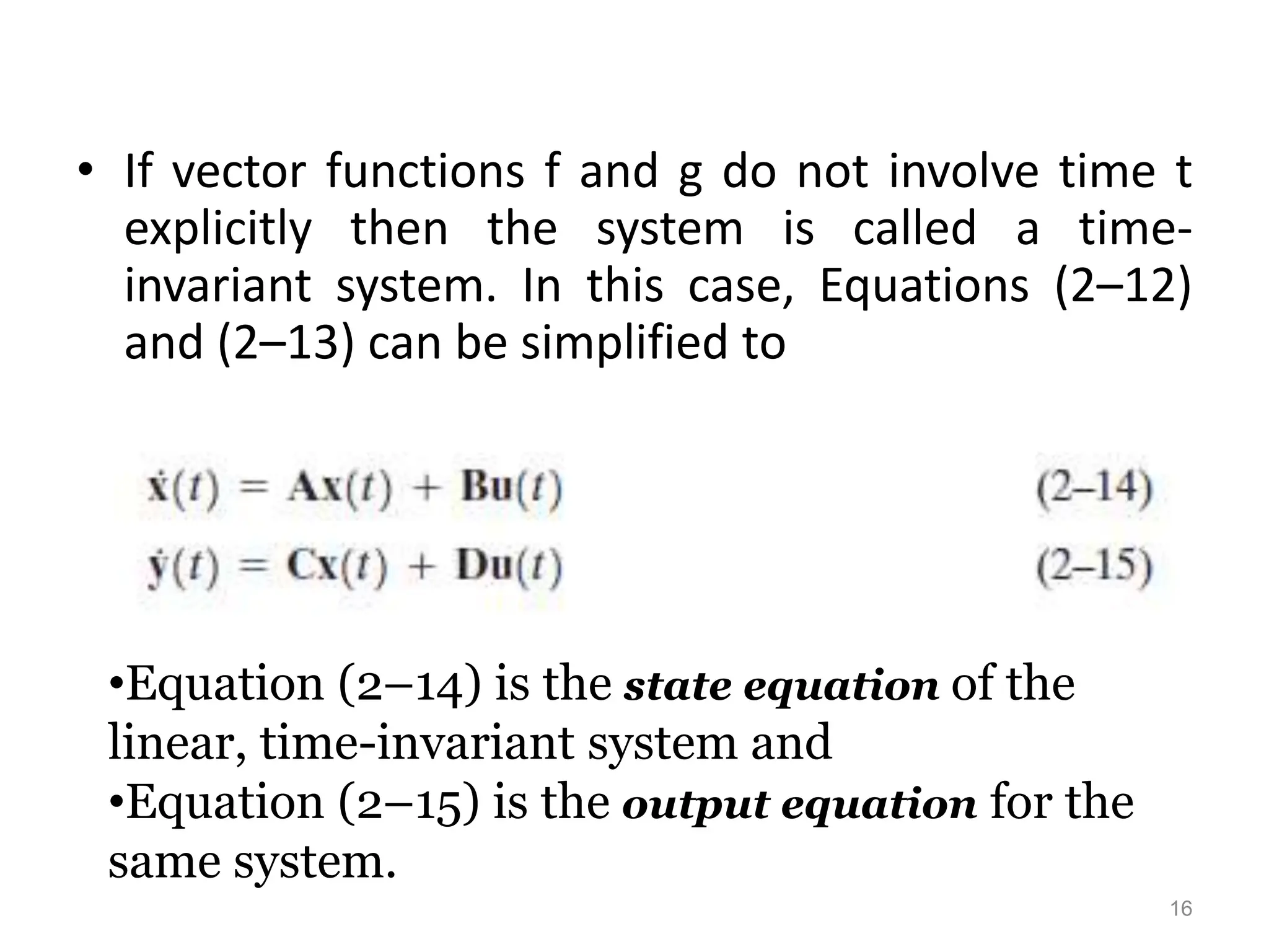
1. There are two main approaches for analyzing and designing control systems: the classical/frequency domain technique using transfer functions and the modern/time domain technique using state-space models. 2. State-space models represent a system using matrices and vectors of input, output, and state variables related by first-order differential equations. This allows analysis of systems with multiple inputs and outputs and knowledge of internal states. 3. A state-space model defines state variables that contain the minimum information needed to describe the system behavior. The state-space is an n-dimensional space with axes defined by the state variables.

1. State Space
1

2. Plant
Mathematical Model :
Differential equation
Linear, time invariant
Frequency Domain
Technique
Time Domain
Technique
Two approaches for analysis and design of control system:
1.Classical Technique or Frequency Domain Technique.(T.F. + graphical plots like root
locus, bode etc.)
2.Modern Technique or Time Domain Technique (State variable approach).
2

3. Transfer Function form
Need of conversion of transfer function form into state space form:
1. In state variable we have so many design techniques available for system. Hence
in order to apply these techniques T.F. must be realized into state variable model.
4
3

4. 4

5. State-Space Modeling
• Uses matrices and vectors to represent the
system parameters and variables
• In control engineering, a state space
representation is a mathematical model of a
physical system as a set of input, output and state
variables related by first-order differential
equations.
5

6. Motivation for State-Space Modeling
Easier for computers to perform matrix
algebra
◦ e.g. MATLAB does all computations as matrix math
Handles multiple inputs and outputs
Provides more information about the system
◦ Provides knowledge of internal variables (states)
Primarily used in complicated, large-scale
systems
6

7. Definitions
• State: Is the smallest set of variables completely
determines the behavior of the system for any
time t.
• State Variables: Are the variables making up the
smallest set of variables.
7

8. State Space:
• The n-dimensional space whose coordinate
axes consist of the x1 axis, x2 axis, ….., xn axis,
where x1, x2,…… , xn are state variables, is
called a state space.
8

9. • State-Space Equations. In state-space analysis we
are concerned with three types of variables that
are involved in the modeling of dynamic systems:
input variables, output variables, and state
variables.
• The number of state variables to completely
define the dynamics of the system is equal to the
number of integrators involved in the system.
• Assume that a multiple-input, multiple-output
system involves n integrators. Assume also that
there are r inputs u1(t), u2(t),……. ur(t) and m
outputs y1(t), y2(t), …….. ym(t).
9

10. • Define n outputs of the integrators as state variables:
x1(t), x2(t), ……… xn(t). Then the system may be
described by
10

11. • The outputs y1(t), y2(t), ……… ym(t) of the
system may be given by
11

12. • If we define
12

13. • then Equations (2–8) and (2–9) become
• where Equation (2–10) is the state equation and
Equation (2–11) is the output equation. If vector
functions f and/or g involve time t explicitly, then the
system is called a time varying system.
13

14. • If Equations (2–10) and (2–11) are linearized
about the operating state, then we have the
following linearized state equation and output
equation:
14

15.  A(t) is called the state matrix,
 B(t) the input matrix,
 C(t) the output matrix, and
 D(t) the direct transmission matrix.
 A block diagram representation of Equations (2–12) and (2–
13) is shown in Figure
15

16. • If vector functions f and g do not involve time t
explicitly then the system is called a time-
invariant system. In this case, Equations (2–12)
and (2–13) can be simplified to
•Equation (2–14) is the state equation of the
linear, time-invariant system and
•Equation (2–15) is the output equation for the
same system.
16