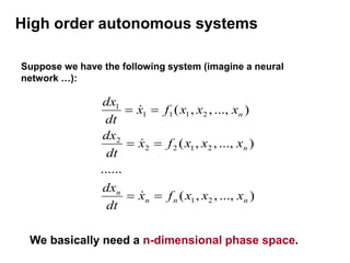
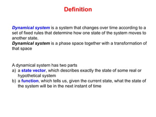
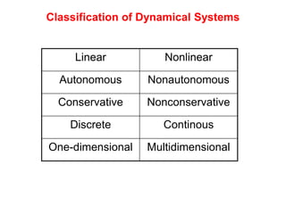
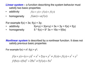
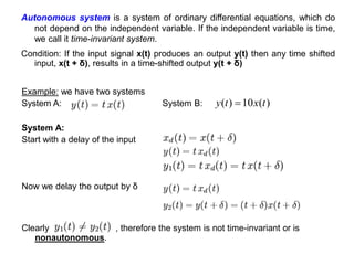
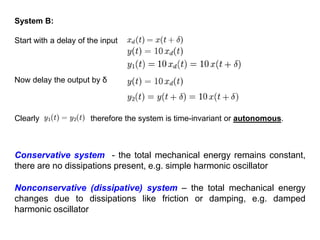
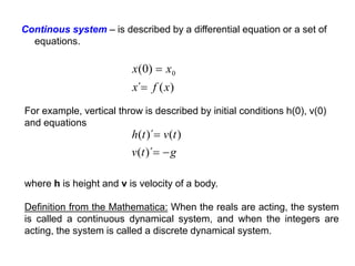
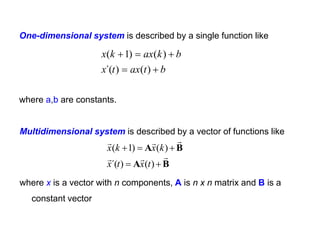
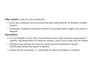
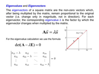
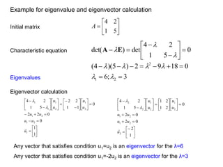
This document defines and describes dynamical systems. It begins by defining a dynamical system as a system that changes over time according to fixed rules determining how its states change. It then describes the two main parts of a dynamical system: (1) a state vector describing the system's current state, and (2) a function determining the next state. Dynamical systems can be classified as linear/nonlinear, autonomous/nonautonomous, conservative/nonconservative, discrete/continuous, and one-dimensional/multidimensional. The document provides examples of classifying systems and calculating eigenvalues and eigenvectors. It discusses how diagonalizing a matrix simplifies solving dynamical systems.

1. Dr.R.Karthikeyan
Professor and Sr.Researcher
Introduction to Dynamical Systems

2. Definition
Dynamical system is a system that changes over time according to a
set of fixed rules that determine how one state of the system moves to
another state.
Dynamical system is a phase space together with a transformation of
that space
A dynamical system has two parts
a) a state vector, which describes exactly the state of some real or
hypothetical system
b) a function, which tells us, given the current state, what the state of
the system will be in the next instant of time

3. A state vector can be described by
)]
(
),......,
(
),
(
[
)
( 2
1 t
x
t
x
t
x
t
x n


)
,....,
,
(
),....,
,....,
,
(
),
,....,
,
( 2
1
2
1
2
2
1
1 n
n
n
n x
x
x
f
x
x
x
f
x
x
x
f
)
,....,
,
(
.
.
)
,....,
,
(
)
,....,
,
(
2
1
2
1
2
2
2
2
1
1
1
1
n
n
n
n
n
n
x
x
x
f
x
dt
dx
x
x
x
f
x
dt
dx
x
x
x
f
x
dt
dx









A function can be described by a single function or by a set of functions
Entire system can be then described by a set of differential equations – equations
of motion

4. Classification of Dynamical Systems
Linear Nonlinear
Autonomous Nonautonomous
Conservative Nonconservative
Discrete Continous
One-dimensional Multidimensional

5. Linear system – a function describing the system behavior must
satisfy two basic properties
• additivity
• homogeneity
)
(
)
(
)
( y
f
x
f
y
x
f 


)
(
)
( x
f
x
f 
 
2
2
2
2
2
2
2
2
5
)
(
5
25
)
5
(
)
5
(
)
(
)
(
2
)
(
)
(
x
x
f
x
x
x
f
y
x
y
f
x
f
y
xy
x
y
x
y
x
f














For example f(x) = 3x; f(y) = 3y;
• additivity f(x+y) = 3(x+y) = 3x + 3y = f(x) + f(y)
• homogeneity 5 * f(x) = 5* 3x = 15x = f(5x)
Nonlinear system is described by a nonlinear function. It does not
satisfy previous basic properties
For example f(x) = x2; f(y) = y2;

6. Example: we have two systems
System A: System B:
Clearly , therefore the system is not time-invariant or is
nonautonomous.
Autonomous system is a system of ordinary differential equations, which do
not depend on the independent variable. If the independent variable is time,
we call it time-invariant system.
Condition: If the input signal x(t) produces an output y(t) then any time shifted
input, x(t + δ), results in a time-shifted output y(t + δ)
)
(
10
)
( t
x
t
y 
System A:
Start with a delay of the input
Now we delay the output by δ

7. Clearly therefore the system is time-invariant or autonomous.
System B:
Conservative system - the total mechanical energy remains constant,
there are no dissipations present, e.g. simple harmonic oscillator
Start with a delay of the input
Now delay the output by δ
Nonconservative (dissipative) system – the total mechanical energy
changes due to dissipations like friction or damping, e.g. damped
harmonic oscillator

8. The system can be solved by iteration calculation. Typical example is annual
progress of a bank account. If the initial deposit is 100000 birr and annual interest
is 3%, then we can describe the system by
)
(
)
(
))
(
(
)
1
(
)
0
(
0
0
x
f
k
x
k
x
f
k
x
x
x
k




100000
*
03
.
1
)
(
)
(
03
.
1
)
1
(
100000
)
0
(
k
k
x
k
x
k
x
x




Discrete system – is described be a difference equation or set of equations. In
case of a single equation we are also talking about one-dimensional map. We
denote time by k, and the system is typically specified by the equations

9. Continous system – is described by a differential equation or a set of
equations.
For example, vertical throw is described by initial conditions h(0), v(0)
and equations
)
(
´
)
0
( 0
x
f
x
x
x


g
t
v
t
v
t
h



)´
(
)
(
)´
(
where h is height and v is velocity of a body.
Definition from the Mathematica: When the reals are acting, the system
is called a continuous dynamical system, and when the integers are
acting, the system is called a discrete dynamical system.

10. Multidimensional system is described by a vector of functions like
where x is a vector with n components, A is n x n matrix and B is a
constant vector
One-dimensional system is described by a single function like
where a,b are constants.
b
t
ax
t
x
b
k
ax
k
x





)
(
)
´(
)
(
)
1
(
B
A
B
A











)
(
)
´(
)
(
)
1
(
t
x
t
x
k
x
k
x

14. Repetition From the Matrix Algebra
Matrix A Matrix B Vector C











33
32
31
23
22
21
13
12
11
a
a
a
a
a
a
a
a
a
A











33
32
31
23
22
21
13
12
11
b
b
b
b
b
b
b
b
b
B











3
2
1
c
c
c
C






























33
33
23
32
13
31
32
33
22
32
12
31
31
33
21
32
11
31
33
23
23
22
13
21
32
23
22
22
12
21
31
23
21
22
11
21
33
13
23
12
13
11
32
13
22
12
12
11
31
13
21
12
11
11
b
a
b
a
b
a
b
a
b
a
b
a
b
a
b
a
b
a
b
a
b
a
b
a
b
a
b
a
b
a
b
a
b
a
b
a
b
a
b
a
b
a
b
a
b
a
b
a
b
a
b
a
b
a
A.B

















3
33
2
32
1
31
3
23
2
22
1
21
3
13
2
12
1
11
c
a
c
a
c
a
c
a
c
a
c
a
c
a
c
a
c
a
C
A.


15. Identity matrix (unit matrix),
we use symbol E or I











1
0
0
0
1
0
0
0
1
E
31
22
13
33
21
12
32
23
11
32
21
13
31
23
12
33
22
11
)
det( a
a
a
a
a
a
a
a
a
a
a
a
a
a
a
a
a
a 





A
32
31
22
21
12
11
33
32
31
23
22
21
13
12
11
a
a
a
a
a
a
a
a
a
a
a
a
a
a
a











A







22
12
21
11
d
d
d
d
D
12
21
22
11
)
det( d
d
d
d 

D
Determinant

16. Inversion matrix – 2x2







d
c
b
a
A
1
1 1 1
det( )
a b d b d b
c d c a c a
ad cb

  
     
  
     
 

     
A
A
Inversion matrix – 3x3

17. u
u




A
For the eigenvalue calculation we use the formula
0
)
det( 
 E
A 
Eigenvalues and Eigenvectors
The eigenvectors of a square matrix are the non-zero vectors which,
after being multiplied by the matrix, remain proportional to the original
vector (i.e. change only in magnitude, not in direction). For each
eigenvector, the corresponding eigenvalue λ is the factor by which the
eigenvector changes when multiplied by the matrix.

18. 0
)
( 
 u

E
A 
For the eigenvector calculation we use the formula:
0
2
1
22
21
12
11















u
u
a
a
a
a


Two-dimensional example:
If we are successful in finding eigenvalues, we can say, that we found a
diagonal matrix, which is similar to the original matrix. The diagonal matrix has
the same properties like the original one for the purpose of solving dynamical
system stability. We write the diagonal matrix in the form:












n



0
0
0
0
...
0
0
0
0
0
0
0
0
2
1

19. What are advantages of diagonal matrix?
1. Multidimensional discrete system.
)
(
)
1
( k
x
k
x


A

 )
0
(
)
( x
k
x k 

A

The typical formula is: To obtain k-th element:
Raising matrices to the power is quite difficult, but in case of diagonal matrix we
simply have:















k
n
k
k
k



0
0
0
0
...
0
0
0
0
0
0
0
0
2
1
A

20. 2. Multidimensional continous system.
)
(t
x
dt
x
d 

A
 )
exp(
)
( 0 t
x
t
x A



The typical differential equation: Solution of the equation:















t
t
t
n
e
e
e
t



0
0
0
0
...
0
0
0
0
0
0
0
0
)
exp(
2
1
A
Using matrices as an argument for the exponential function is much more difficult
than raising them to the power, but in case of diagonal matrix we can write:

21. Example for eigenvalue and eigenvector calculation







5
1
2
4
A










































1
1
0
0
2
2
0
1
1
2
2
5
1
2
4
1
2
1
2
1
2
1
2
1
1
1
u
u
u
u
u
u
u
u
u



Initial matrix







































1
2
0
2
0
2
0
2
1
2
1
5
1
2
4
2
2
1
2
1
2
1
2
1
2
2
u
u
u
u
u
u
u
u
u



Any vector that satisfies condition u1=u2 is an eigenvector for the λ=6
Any vector that satisfies condition u1=-2u2 is an eigenvector for the λ=3
Characteristic equation
Eigenvalues
Eigenvector calculation
0
5
1
2
4
det
)
det( 












E
A
3
;
6
0
18
9
2
)
5
)(
4
(
2
1
2
















22. Trace of a matrix is a sum of the elements on the main diagonal
nn
a
a
a
Tr 


 ....
)
( 22
11
A
)
,....,
,
(
.
.
)
,....,
,
(
)
,....,
,
(
2
1
2
1
2
2
2
2
1
1
1
1
n
n
n
n
n
n
x
x
x
f
x
dt
dx
x
x
x
f
x
dt
dx
x
x
x
f
x
dt
dx
















































n
n
n
n
n
n
x
f
x
f
x
f
x
f
x
f
x
f
x
f
x
f
x
f
...
...
...
...
...
...
2
1
2
2
2
1
2
1
2
1
1
1
J
Jacobian matrix is the matrix of all first-order partial derivatives of a vector-
or scalar-valued function with respect to another vector. This matrix is
frequently being marked as J, Df or A.

23. Phase Portraits
A phase space is a space in which all possible states of a system are
represented, with each possible state of the system corresponding
to one unique point in the phase space.
The phase space of a two-dimensional system is called a phase plane,
which occurs in classical mechanics for a single particle moving in
one dimension, and where the two variables are position and
velocity.
For mechanical systems, the phase space usually consists of all
possible values of position and velocity variables. A plot of position
and velocity variables as a function of time is sometimes called a
phase diagram.
A phase portrait is a plot of single phase curve or multiple phase
curves corresponding to different initial conditions in the same phase
plane.

24. A phase portrait of a simple harmonic oscillator
Differential equation
)
sin(
)
cos(
t
A
v
t
A
x





)
(
sin
)
(
cos
2
2
2
2
t
A
v
t
A
x

















0
2

 x
x 


)
sin(
)
cos(
t
A
v
t
A
x






Now we separate sine and cosine functions, raise both equations to the power
of two and finally we add them.
where x is displacement, v is
velocity, A is amplitude
and ω is angular frequency.
1
)
(
sin
)
(
cos 2
2
2
2
















t
t
A
v
A
x



1
2
2














A
v
A
x

Final equation describes an ellipse
Solution of the equation

25. The following figure shows a phase portrait of a simple harmonic oscillator
with ω=10 s-1 and initial conditions x(0)=1 m; v(0)=0 m/s
1
10
1
2
2













 v
x
1
2
2














A
v
A
x


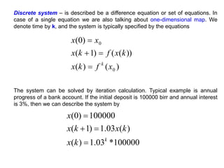
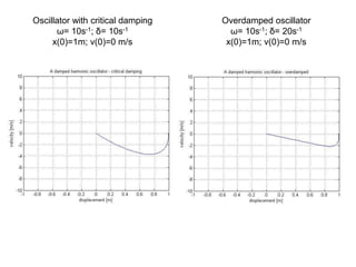
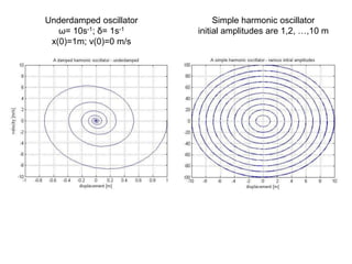
26. Creating a phase portrait of a damped oscillator in Matlab
function [t,y] = oscil(delta)
tspan=[0,7];
init=[1;0];
omega=10;
[t,y]=ode45(@f,tspan,init);
plot(y(:,1),y(:,2));
%Creation of graph description.
xlabel('displacement [m]')
ylabel('velocity [m/s]')
title('A damped harmonic oscillator');
axis([-1 1 -10 10]);
function yprime=f(t,y)
yprime=zeros(2,1);
yprime(1)=y(2);
yprime(2)=-2*delta*y(2)-omega^2*y(1);
end
clc
end
y
y
y
y
y
y
2
2
2
0
2
















y
y
y
y



2
1
y
y
y
y
y
y
2
2
1
2 
 










0
)
0
(
)
0
(
1
)
0
(
)
0
(
2
1




y
y
y
y

1
2
2
2
2
1
2 y
y
y
y
y

 






27. Oscillator with critical damping
ω= 10s-1; δ= 10s-1
x(0)=1m; v(0)=0 m/s
Overdamped oscillator
ω= 10s-1; δ= 20s-1
x(0)=1m; v(0)=0 m/s

28. Underdamped oscillator
ω= 10s-1; δ= 1s-1
x(0)=1m; v(0)=0 m/s
Simple harmonic oscillator
initial amplitudes are 1,2, …,10 m

29. Equilibria of a dynamical system
Coin balanced on a table
－How many equilibria? (Face Up, Face Down, Edge)
－ Is it stable?
A ball in the track:
It’s either on top of a hill or at the bottom of the track. To find
out which, push it (perturb it), and see if it comes back.

30. Fixed points of First-order autonomous
systems
0
)
,
( 
 
x
f
dt
dx
)
,
,
( t
x
f
x
dt
dx


 
By a fixed point we mean that x doesn’t change as time
increases, i.e.:
So, to find fixed points just solve above equation.
)
,
( 
x
f
dt
dx

autonomous systems
nonautonomous systems

31. E.g.: dx/dt = Ax(1 – x) with A=6. What are the fixed
points?
Set: dx/dt = 0 ie: 6x(1-x) = 0
so either x = 0 or x = 1
Use difference equation: x(t+h) = x(t) +h dx/dt from various
different initial values of x
Therefore 2 fixed points, and how about the stability?
Perturb the points and see what happens under the system
dynamics…

32. Vector fields
0 0.5 1 1.5
0
0.1
0.2
0.3
0.4
0.5
0.6
0.7
0.8
0.9
1
t
x
(t, x(t))
(t+h, x(t)+hdx/dt)
So x=0 is unstable and x=1 seems to be stable.
Change the value of parameter A to see the influence of
parameters on systems

33. Phase flow in 1-D phase space
)
1
( x
Ax
x
dt
dx


 
hdx/dt
1-D phase space
dt
dx

34. First-order autonomous systems






0
0
)
,
(
dx
x
df k 
)
,
( 
x
f
dt
dx

1. Find fixed points:
2. Identify stability
－using phase flow as above
－using the gradient at the fixed points
xk is stable
xk is unstable
0
)
,
( 

k
x
f

35. Exercise 1:
a
dx
ax
d

)
(
1. Fixed points: x=0
2. Stable or not?
If a<0, d(ax)/dx<0. stable
ax
dt
dx

If a>0, d(ax)/dx>0. unstable

36. Exercise 2: 3
x
x
dt
dx



1
3
)
( 2
3




x
dx
x
x
d
1. Fixed points: x=0, +1, -1
2. Stable or not?

37. Second-order autonomous systems
)
,
(
)
,
(
y
x
g
y
dt
dy
y
x
f
x
dt
dx






Suppose we have the following system:
1. Find the fixed points by setting:
0
)
,
(
0
)
,
(


k
k
k
k
y
x
g
y
x
f
2. Identify stability by Jacobian matrix (will not talk here) or
2-D phase space portrait

38. Phase space portrait
The 2-D space of possible initial conditions in which each
solution follows a trajectory given by the vector field
(x(t+h),y(t+h)) =(x(t)+hdx/dt, y(t)+hdy/dt)
(x(t),y(t))
x
y
)
,
(
)
,
(
y
x
g
y
dt
dy
y
x
f
x
dt
dx







39. Classification of Dynamical Systems
Two-dimensional linear or linearized systems
2
1
2
1
2
2
2
1
2
1
1
1
)
,
(
)
,
(
dx
cx
x
x
f
x
bx
ax
x
x
f
x



































d
c
b
a
x
f
x
f
x
f
x
f
2
2
1
2
2
1
1
1
A
J
0
)
(
0
)
)(
(
0
det
0
)
det(
2






















bc
ad
d
a
bc
d
a
d
c
b
a






E
A
Set of equations for 2D system
Jacobian matrix for 2D system
Calculation of eigenvalues
2
)
(
4
)
(
)
(
0
)
(
)
(
)
(
;
)
(
2
12
2
A
A
A
A
A
A
A
Det
Tr
Tr
Det
Tr
bc
ad
Det
d
a
Tr













Formulation using trace and
determinant

40. Types of two-dimensional linear systems
1. Attracting Node (Sink)
2
2
1
1
4x
x
x
x















4
0
0
1
A
Equations
Jacobian matrix
Eigenvalues
λ1= -1
λ2= -4
Conclusion: there is a stable fixed point, the node-sink
Eigenvectors












1
0
0
1

41. 2. Repelling Node
2
2
1
1
4x
x
x
x




Equations
Jacobian matrix
Eigenvalues
λ1= 1
λ2= 4







4
0
0
1
A
Conclusion: there is an unstable fixed point, the repelling node
Eigenvectors












1
0
0
1

42. 3. Saddle Point
2
2
1
1
4x
x
x
x





Equations
Jacobian matrix
Eigenvalues
λ1= -1
λ2= 4







4
0
0
1
A
Conclusion: there is an unstable fixed point, the saddle point
Eigenvectors












1
0
0
1

43. 4. Spiral Source (Repelling Spiral)
2
1
2
2
1
1
2
2
x
x
x
x
x
x







Equations
Jacobian matrix
Eigenvalues
λ1= 1+2i
λ2= 1-2i








1
2
2
1
A
Conclusion: there is an unstable fixed point, the spiral source
sometimes called unstable focal point
Eigenvectors












1
1
i
i

44. 5. Spiral Sink
2
1
2
2
1
1
2
2
x
x
x
x
x
x








Equations
Jacobian matrix
Eigenvalues
λ1= -1+2i
λ2= -1-2i










1
2
2
1
A
Conclusion: there is a stable fixed point, the spiral sink
sometimes called stable focal point
Eigenvectors












1
1
i
i

45. 6. Node Center
2
1
2
2
1
1
4 x
x
x
x
x
x







Equations
Jacobian matrix
Eigenvalues
λ1= +1.732i
λ2= -1.732i





 


1
4
1
1
A
Conclusion: there is marginally stable (neutral) fixed point, the node center
Eigenvectors





 






 

1
43
.
0
25
.
0
1
43
.
0
25
.
0 i
i

46. Brief classification of two-dimensional dynamical systems according to
eigenvalues

47. Special cases of identical eigenvalues
2
2
1
1
x
x
x
x















1
0
0
1
A












0
1
1
0
1
12 


t
t
e
x
x
e
x
x 20
2
10
1 ; 

Equations
and matrix
Eigenvalues +
eigenvectors
2
2
1
1
x
x
x
x











1
0
0
1
A












0
1
1
0
1
12 


Equations
and matrix
Eigenvalues +
eigenvectors
t
t
e
x
x
e
x
x 


 20
2
10
1 ;
Solution
Solution
A stable star (a stable proper node)
An unstable star (an unstable proper node)

48. Special cases of identical eigenvalues
2
2
2
1
1
x
x
x
x
x
















1
0
1
1
A












0
0
0
1
1
12 


t
t
e
x
x
e
tx
x
x 20
2
20
10
1 ;
)
( 


Equations
and matrix
Eigenvalues +
eigenvectors
2
2
2
1
1
x
x
x
x
x












1
0
1
1
A












0
0
0
1
1
12 


Equations
and matrix
Eigenvalues +
eigenvectors
t
t
e
x
x
e
tx
x
x 



 20
2
20
10
1 ;
)
(
Solution
Solution
A stable improper node with 1 eigenvector
An unstable improper node with 1 eigenvector

49. 2
4
2
)
(
4
)
(
)
( 2
2
12
q
p
p
Det
Tr
Tr 





A
A
A

Classification of dynamical systems using
trace and determinant of the Jacobian matrix
1.Attracting node
p=-5; q=4; Δ=9
2. Repelling node
p=5; q=4; Δ=9
3. Saddle point
p=3; q=-4; Δ=25
4. Spiral source
p=2; q=5; Δ=-16
5. Spiral sink
p=-2; q=5; Δ=-16
6. Node center
p=0; q=5; Δ=-20
7. Stable/unstable star
p=-/+ 2; q=1; Δ=0
8. Stable/unstable
improper node
p=-/+ 2; q=1; Δ=0

50. Classification of Dynamical Systems
Linear or linearized systems with more dimensions
Time Eigenvalues Fixed point is
Continous
all Re(λ)<0 Stable
some Re(λ)>0 Unstable
all Re(λ)<=0
some Re(λ)=0
Cannot decide
Discrete
all |λ|<1 Stable
some |λ|>1 Unstable
all |λ|<=1
some |λ|=1
Cannot decide

51. Example 1: A damped simple pendulum

52. A damped simple pendulum
)
0
(
0
)
sin(
2
2




a
dt
d
a
dt
d




53. Second-order autonomous systems
First-order autonomous system in two variables
)
sin( x
ay
dt
dy
y
dt
dx




dt
d
y
x

 
 ,
Find the fixed points: (0, 0), (±π, 0), ……
)
0
(
0
)
sin(
2
2




a
dt
d
a
dt
d




54. Phase space portrait of the damped simple
pendulum
)
sin(
4
.
0 x
y
dt
dy
y
dt
dx





55. Example 2: the Van der Pol oscillator

56. Van der Pol oscillator
0
)
1
( 2
2
2



 x
dt
dx
x
t
d
x
d

The second term is not a constant like that in the damped simple
pendulum with )
0
(
,
0
)
sin( 


 a
a 

 


Second-order autonomous systems
first-order autonomous system in two variables
x
y
x
dt
dy
y
dt
dx





)
1
( 2

dt
dx
y 

57. Find the fixed points: (0, 0). Stable or not?
x
y
x
dt
dy
y
dt
dx





)
1
( 2

Phase space portrait
with λ = 1.

58. The Limit Cycle

59. High order autonomous systems
)
...,
,
,
(
......
)
...,
,
,
(
)
...,
,
,
(
2
1
2
1
2
2
2
2
1
1
1
1
n
n
n
n
n
n
x
x
x
f
x
dt
dx
x
x
x
f
x
dt
dx
x
x
x
f
x
dt
dx









Suppose we have the following system (imagine a neural
network …):
We basically need a n-dimensional phase space.

60. Stability and Fixed Points
A fixed point is a special point of the dynamical system which does not
change in time. It is also called an equilibrium, steady-state, or singular point of
the system.
If a system is defined by an equation dx/dt = f(x), then the fixed point x~ can be
found by examining of condition f(x~)=0. We need not know analytic solution of
x(t).
For discrete time systems we examine condition x~ = f(x~)
An attractor is a set towards which a dynamical system evolves over time. It
can be a point, a curve or more complicated structure
A stable fixed point: for all starting values x0 near the x~ the system converges
to the x~ as t→∞.
A marginally stable (neutral) fixed point: for all starting values x0 near x~, the
system stays near x~ but does not converge to x~ .
An unstable fixed point: for starting values x0 very near x~ the system moves
far away from x~
A perturbation is a small change in a physical system, most often in a physical
system at equilibrium that is disturbed from the outside.

61. Phase portraits of basic three types of fixed points
STABLE MARGINALLY STABLE UNSTABLE

63. Both positive Nodal Source Unstable
Both Negative Nodal sink Stable
Opposite signs Saddle points Unstable
Real Eigen values
Complex Eigen values
Positive real parts Spiral Source Unstable
Negative real parts Spiral sink Stable
Zero real parts Inconclusive for Nonlinear
system
Center for Linear system
Unstable

65. What can we do if linearization method cannot decide?
Unusually damped harmonic oscillator
We have a harmonic oscillator, where the mass m
moves in very viscous medium, where the damping
force is proportional to the cube of the velocity.
3
v
x
v
v
x















v
x
y
where
y
f
y




),
( 














 3
)
(
v
x
v
v
x
f
y
f


Set of differential equations
describing the system
After setting vector variable y we can write
Fixed point result from equations
0
0
3




v
x
v
 






0
0
~
y

There is only one fixed point

66. The Jacobian matrix








 2
3
1
1
0
v
f

D 3
v
x
v
v
x







Jacobian matrix for linearized
system at the fixed point 







0
1
1
0
)
~
(y
f

D
Eigenvalues for this system are λ12= +/- i, so they have zero real part and the
method of linearization cannot decide about the stability.
The graph shows phase diagram
for μ=0.25, x0=2 and v0=0.
Even from the graph it is not clear
if the trajectory will converge to
(0,0) point or if it will remain at
certain non-zero distance from it.
We will have to use another tool –
Lyapunov functions which we
will see in the forth coming
classes