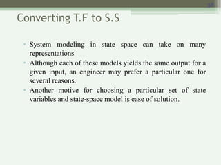
This document discusses state space representation of systems. It begins by outlining how to find a state space model for a linear time-invariant system using state equations and matrices. It then provides examples of deriving state space models for electrical, mechanical, and electromechanical systems. The document also covers converting between transfer functions and state space models, and defines key terms like state vector, state space, controllability, and observability.

1. State Space Representation of
System
Dr.Ziad Saeed Mohammed
E .T .C-N.T.U
2019-2020

2. outline
• How to find mathematical model, called a state-
space representation, for a linear, time-invariant
system
• How to convert between transfer function and
state space models

3. Modeling
3
Derive mathematical models for
• Electrical systems
• Mechanical systems
• Electromechanical system
Electrical Systems:
• Kirchhoff’s voltage & current laws
Mechanical systems:
• Newton’s laws

4. 4
State-Space Modeling
• Alternative method of modeling a system than
▫ Differential / difference equations
▫ Transfer functions
• Uses matrices and vectors to represent the system
parameters and variables
• In control engineering, a state space
representation is a mathematical model of a
physical system as a set of input, output and state
variables related by first-order differential
equations. To abstract from the number of inputs,
outputs and states, the variables are expressed as
vectors.

5. 5
Motivation for State-Space Modeling
• Easier for computers to perform matrix algebra
▫ e.g. MATLAB does all computations as matrix math
• Handles multiple inputs and outputs
• Provides more information about the system
▫ Provides knowledge of internal variables (states)
Primarily used in complicated, large-scale
systems

6. State space model composed of 2 equations;
1. State equation
State
Space Model
2. Output equation
6
• A is called the state matrix,
• B the input matrix,
• C the output matrix, and
• D the direct transmission matrix.

7. Definitions
• State- The state of a dynamic system is the
smallest set of variables (called state variables)
such that knowledge of these variables at t=t0 ,
together with knowledge of the input for t ≥ t0 ,
completely determines the behavior of the
system for any time t to to.
• Note that the concept of state is by no means
limited to physical systems. It is applicable to
biological systems, economic systems, social
systems, and others.

8. State Variables:
• The state variables of a dynamic system are the
variables making up the smallest set of variables
that determine the state of the dynamic system.
• If at least n variables x1, x2, …… , xn are needed
to completely describe the behavior of a
dynamic system (so that once the input is given
for t ≥ t0 and the initial state at t=to is specified,
the future state of the system is completely
determined), then such n variables are a set of
state variables.

9. State Vector:
• A vector whose elements are the state variables.
• If n state variables are needed to completely
describe the behavior of a given system, then
these n state variables can be considered the n
components of a vector x. Such a vector is called
a state vector.
• A state vector is thus a vector that determines
uniquely the system state x(t) for any time t≥ t0,
once the state at t=t0 is given and the input u(t)
for t ≥ t0 is specified.

10. State Space:
• The n-dimensional space whose coordinate axes
consist of the x1 axis, x2 axis, ….., xn axis, where
x1, x2,…… , xn are state variables, is called a
state space.
• "State space" refers to the space whose axes are
the state variables. The state of the system can
be represented as a vector within that space.

11. • State-Space Equations. In state-space analysis
we are concerned with three types of variables
that are involved in the modeling of dynamic
systems: input variables, output variables, and
state variables.
• The number of state variables to completely
define the dynamics of the system is equal to the
number of integrators involved in the system.
• Assume that a multiple-input, multiple-output
system involves n integrators. Assume also that
there are r inputs u1(t), u2(t),……. ur(t) and m
outputs y1(t), y2(t), …….. ym(t).

12. • Define n outputs of the integrators as state variables:
x1(t), x2(t), ……… xn(t). Then the system may be
described by:

13. • The outputs y1(t), y2(t), ……… ym(t) of the
system may be given by

14. • If we define

15. • then Equations (2–8) and (2–9) become
• where Equation (2–10) is the state equation and
Equation (2–11) is the output equation. If vector
functions f and/or g involve time t explicitly, then the
system is called a time varying system.

16. • If Equations (2–10) and (2–11) are linearized
about the operating state, then we have the
following linearized state equation and output
equation:

17. • A(t) is called the state matrix,
• B(t) the input matrix,
• C(t) the output matrix, and
• D(t) the direct transmission matrix.
• A block diagram representation of Equations (2–12) and
(2–13) is shown in Figure

18. • If vector functions f and g do not involve time t
explicitly then the system is called a time-
invariant system. In this case, Equations (2–12)
and (2–13) can be simplified to
•Equation (2–14) is the state equation of the
linear, time-invariant system and
•Equation (2–15) is the output equation for the
same system.

19. Correlation Between Transfer Functions
and State-Space Equations
• The "transfer function" of a continuous time-
invariant linear state-space model can be derived
in the following way:
First, taking the Laplace transform of
Yields

26. Example
26
Find state model of
System shown in the Fig.
Solution
• A practical approach is to assign the current in the inductor L, i(t), and
the voltage across the capacitor C, ec(t), as the state variables.
• The reason for this choice is because the state variables are directly
related to the energy-storage element of a system. The inductor stores
kinetic energy, and the capacitor stores electric potential energy.
• By assigning i(t) and ec(t) as state variables, we have a complete
description of the past history (via the initial states) and the present and
future states of the network.

27. Example
The state equation:
27
This format is also known as the state form if we set
OR

28. Example
28
write the state equations of the electric network shown in the Fig.
Solution: The state equations of the network are obtained by writing the
voltages across the inductors and the currents in the capacitor in terms of the three
state variables. The state equations are

29. Example
In vector-matrix form, the state equations are written as
29
Where

30. Example 3.1 P.138
PROBLEM: Given the electrical network of Figure shown, find
a state-space representation if the output is the current through
the resistor.
30
Solution
Select the state variables by writing the derivative equation for all energy storage
elements, that is, the inductor and the capacitor. Thus,
1
2

31. Example 3.1
Apply network theory, such as Kirchhoffs voltage and current
laws, to obtain ic and vL in terms of the state variables, vc and iL.
At Node 1,
31
which yields ic in terms of the state variables, vc and iL . Around the outer
loop,
3
4

32. Example 3.1
Substitute the results of Eqs. (3) and (4) into Eqs. (1) and (2) to
obtain the following state equations:
32
OR
Find the output eq. since the output is iR(t)
The final result for the state-space representation is

33. Example
33
Find the state eq. of the
mechanical system shown
Solution

34. Example 3.3 P.142
PROBLEM: Find the state equations for the translational
mechanical system shown in Figure.
34

35. Example 3.3 P.142
SOLUTION: First write the differential equations for the
network in Figure, using the methods of Chapter 2 to find the
Laplace-transformed equations of motion.
35

36. Example 3.3 P.142
36
In Vector Matrix

37. 3.5 Converting a Transfer Function to State
Space
In the last section, we applied the state-space representation to
electrical and mechanical systems. We learn how to convert a
transfer function representation to a state-space representation in
this section.
One advantage of the state-space representation is that it can be
used for the simulation of physical systems on the digital
computer. Thus, if we want to simulate a system that is
represented by a transfer function, we must first convert the
transfer function representation to state space.
37

38. Converting T.F to S.S
• System modeling in state space can take on many
representations
• Although each of these models yields the same output for a
given input, an engineer may prefer a particular one for
several reasons.
• Another motive for choosing a particular set of state
variables and state-space model is ease of solution.
38

39. 3.6 Converting from State Space to a
Transfer Function
•
39

40. Converting From S.S to T.F
•
40

41. CONTROLLABILITY:
Full-state feedback design commonly relies on pole-placement
techniques. It is important to note that a system must be completely
controllable and completely observable to allow the flexibility to place all
the closed-loop system poles arbitrarily. The concepts of controllability and
observability were introduced by Kalman in the 1960s.
A system is completely controllable if there exists an unconstrained
control u(t) that can transfer any initial state x(t0) to any other desired
location x(t) in a finite time, t0≤t≤T.

42. For the system
Bu
Ax
x 


we can determine whether the system is controllable by examining the
algebraic condition
  n
B
A
B
A
AB
B
rank 1
n
2



The matrix A is an nxn matrix an B is an nx1 matrix. For multi input systems,
B can be nxm, where m is the number of inputs.
For a single-input, single-output system, the controllability matrix Pc is
described in terms of A and B as
 
B
A
B
A
AB
B
P 1
n
2
c

 
which is nxn matrix. Therefore, if the determinant of Pc is nonzero, the system
is controllable.

43. Example:
Consider the system
   u
0
x
0
0
1
y
,
u
1
0
0
x
a
a
a
1
0
0
0
1
0
x
2
1
0




























 

















































1
2
2
2
2
2
2
1
0 a
a
a
1
B
A
,
a
1
0
AB
,
1
0
0
B
,
a
a
a
1
0
0
0
1
0
A
 
 














1
2
2
2
2
2
c
a
a
a
1
a
1
0
1
0
0
B
A
AB
B
P
The determinant of Pc =1 and ≠0 , hence this system is controllable.

44. Example.
Consider a system represented by the two state equations
1
2
2
1
1 x
d
x
3
x
,
u
x
2
x 




 

The output of the system is y=x2. Determine the condition of controllability.
   u
0
x
1
0
y
,
u
0
1
x
3
d
0
2
x 























 






























d
0
2
1
P
d
2
0
1
3
d
0
2
AB
and
0
1
B
c The determinant of pc is equal to d, which is
nonzero only when d is nonzero.
Dorf and Bishop, Modern Control Systems

45. OBSERVABILITY:
All the poles of the closed-loop system can be placed arbitrarily in the complex
plane if and only if the system is observable and controllable. Observability
refers to the ability to estimate a state variable.
A system is completely observable if and only if there exists a finite time T
such that the initial state x(0) can be determined from the
observation history y(t) given the control u(t).
Cx
y
and
Bu
Ax
x 



Consider the single-input, single-output system
where C is a 1xn row vector, and x is an nx1 column vector. This system is
completely observable when the determinant of the observability matrix P0
is nonzero.

46. The observability matrix, which is an nxn matrix, is written as













1
n
O
A
C
A
C
C
P

Example:
Consider the previously given system
 
0
0
1
C
,
a
a
a
1
0
0
0
1
0
A
2
1
0















Dorf and Bishop, Modern Control Systems

47.    
1
0
0
CA
,
0
1
0
CA 2


Thus, we obtain











1
0
0
0
1
0
0
0
1
PO
The det P0=1, and the system is completely observable. Note that
determination of observability does not utility the B and C matrices.
Example: Consider the system given by
 x
1
1
y
and
u
1
1
x
1
1
0
2
x 


















48. We can check the system controllability and observability using the Pc and P0
matrices.
From the system definition, we obtain
















2
2
AB
and
1
1
B
  









2
1
2
1
AB
B
Pc
Therefore, the controllability matrix is determined to be
det Pc=0 and rank(Pc)=1. Thus, the system is not controllable.
  









2
1
2
1
AB
B
Pc
Therefore, the controllability matrix is determined to be
Dorf and Bishop, Modern Control Systems

49. From the system definition, we obtain
   
1
1
CA
and
1
1
C 















1
1
1
1
CA
C
Po
Therefore, the observability matrix is determined to be
det PO=0 and rank(PO)=1. Thus, the system is not observable.
If we look again at the state model, we note that
2
1 x
x
y 

However,
  2
1
1
2
1
2
1 x
x
u
u
x
x
x
2
x
x 






 


50. Thus, the system state variables do not depend on u, and the system is not
controllable. Similarly, the output (x1+x2) depends on x1(0) plus x2(0) and does
not allow us to determine x1(0) and x2(0) independently. Consequently, the
system is not observable.
The observability matrix PO can be constructed in Matlab by using obsv
command.
From two-mass system,
Po =
1 1
1 1
rank_Po =
1
det_Po =
0
clc
clear
A=[2 0;-1 1];
C=[1 1];
Po=obsv(A,C)
rank_Po=rank(Po)
det_Po=det(Po) The system is not
observable.
Dorf and Bishop, Modern Control Systems