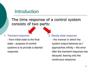
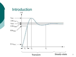
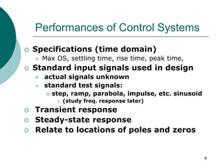
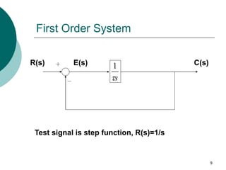
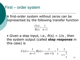
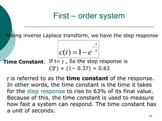
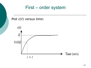
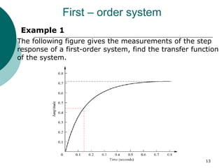
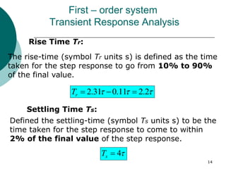
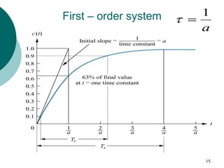
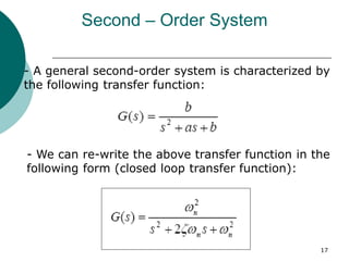
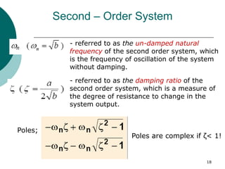
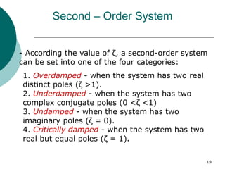
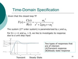
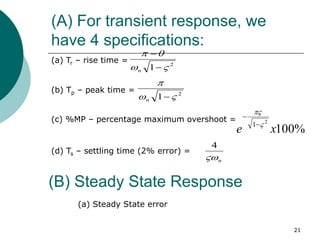
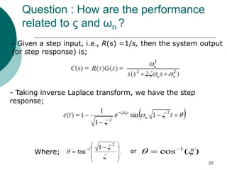
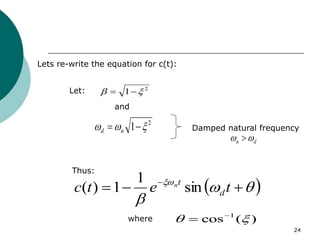
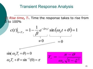
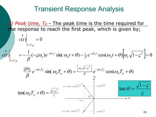
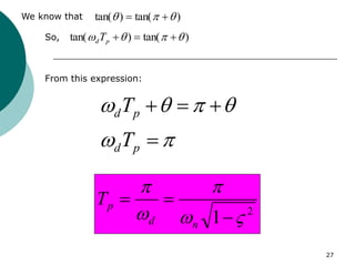
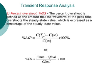
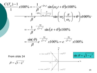
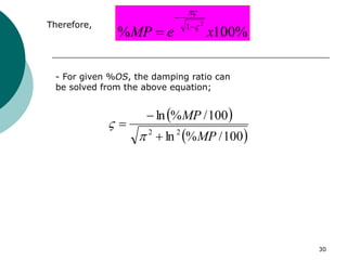
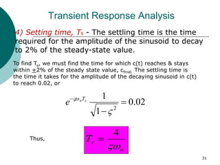
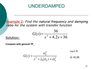
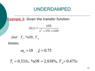
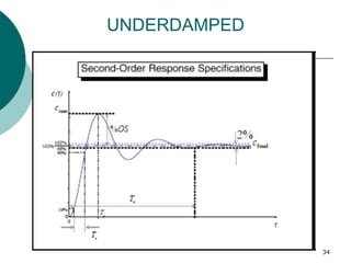
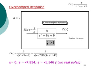
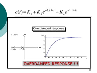
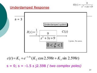
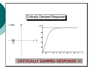
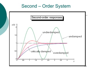
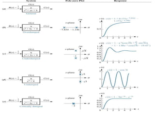
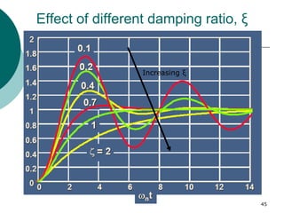
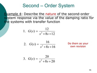
1
Transient & Steady State Response
Analysis
Time Response Analysis
2
Previous Class
 In previous Chapter :
 Block diagram reduction
 Signal flow graphs (SFGs)
Transfer Function
Today’s class
 Transient & Steady State Response
Analysis
 First Order System
 Second Order System
3
Learning Outcomes
 At the end of this lecture, students
should be able to:
 Identify between transient response &
steady state response
 Obtain the transfer function for a first
order system based on graph analysis
 To become familiar with the wide range
of response for second order systems
4
5
In thisChapter
What you are expected to learn :
First order system
Second order system
Routh-Hurwitz Criterion
Steady-state error
Chapter 4
6
Introduction
The time response of a control system
consists of two parts:
1. Transient response
- from initial state to the final
state – purpose of control
systems is to provide a desired
response.
2. Steady-state response
- the manner in which the
system output behaves as t
approaches infinity – the error
after the transient response has
decayed, leaving only the
continuous response.
7
Introduction
Transient Steady-state
8
Performances of Control Systems
 Specifications (time domain)
 Max OS, settling time, rise time, peak time,
 Standard input signals used in design
 actual signals unknown
 standard test signals:
 step, ramp, parabola, impulse, etc. sinusoid
 (study freq. response later)
 Transient response
 Steady-state response
 Relate to locations of poles and zeros
9
First Order System
s

1
R(s) C(s)
E(s)
Test signal is step function, R(s)=1/s
10
First – order system
1
1
)
(
)
(


s
s
R
s
C

A first-order system without zeros can be
represented by the following transfer function
• Given a step input, i.e., R(s) = 1/s , then
the system output (called step response in
this case) is


 1
1
1
)
1
(
1
)
(
1
1
)
(







s
s
s
s
s
R
s
s
C
11
First – order system

t
e
t
c


1
)
(
Taking inverse Laplace transform, we have the step response
Time Constant: If t= , So the step response is
C( ) = (1− 0.37) = 0.63

is referred to as the time constant of the response.
In other words, the time constant is the time it takes
for the step response to rise to 63% of its final value.
Because of this, the time constant is used to measure
how fast a system can respond. The time constant has
a unit of seconds.





12
First – order system
Plot c(t) versus time:
13
The following figure gives the measurements of the step
response of a first-order system, find the transfer function
of the system.
First – order system
Example 1
14
First – order system
Transient Response Analysis
Rise Time Tr:
The rise-time (symbol Tr units s) is defined as the time
taken for the step response to go from 10% to 90%
of the final value.
Settling Time Ts:
Defined the settling-time (symbol Ts units s) to be the
time taken for the step response to come to within
2% of the final value of the step response.


 2
.
2
11
.
0
31
.
2 


r
T

4

s
T
15
First – order system
a
1


16
Second – Order System
 Second-order systems exhibit a wide range of
responses which must be analyzed and described.
• Whereas for a first-order system, varying a
single parameter changes the speed of response,
changes in the parameters of a second order
system can change the form of the response.
 For example: a second-order system can display
characteristics much like a first-order system or,
depending on component values, display damped
or pure oscillations for its transient response.
17
Second – Order System
- A general second-order system is characterized by
the following transfer function:
- We can re-write the above transfer function in the
following form (closed loop transfer function):
18
Second – Order System
- referred to as the un-damped natural
frequency of the second order system, which
is the frequency of oscillation of the system
without damping.
- referred to as the damping ratio of the
second order system, which is a measure of
the degree of resistance to change in the
system output.
Poles;
Poles are complex if ζ< 1!
19
Second – Order System
- According the value of ζ, a second-order system
can be set into one of the four categories:
1. Overdamped - when the system has two real
distinct poles (ζ >1).
2. Underdamped - when the system has two
complex conjugate poles (0 <ζ <1)
3. Undamped - when the system has two
imaginary poles (ζ = 0).
4. Critically damped - when the system has two
real but equal poles (ζ = 1).
Time-Domain Specification
20
2
2
2
2
)
(
)
(
)
(
n
n
n
s
s
s
R
s
C
s
T







Given that the closed loop TF
The system (2nd order system) is parameterized by ς and ωn
For 0< ς <1 and ωn > 0, we like to investigate its response
due to a unit step input
Transient Steady State
Two types of responses that
are of interest:
(A)Transient response
(B)Steady state response
(A) For transient response, we
have 4 specifications:
21
(a) Tr – rise time =
(b) Tp – peak time =
(c) %MP – percentage maximum overshoot =
(d) Ts – settling time (2% error) =
2
1 





n
2
1 



n
%
100
2
1
x
e 



n

4
(B) Steady State Response
(a) Steady State error
22
Question : How are the performance
related to ς and ωn ?
- Given a step input, i.e., R(s) =1/s, then the system output
(or step response) is;
- Taking inverse Laplace transform, we have the step
response;
Where; or )
(
cos 1

 

23
Second – Order System
Mapping the poles into s-plane
2
2
2
2
)
(
)
(
)
(
n
n
n
s
s
s
R
s
C
s
T







24
Lets re-write the equation for c(t):
Let: 2
1 
 

2
1 

 
 n
d
and
Damped natural frequency
d
n 
 
Thus:
 






 
t
e
t
c d
t
n
sin
1
1
)
(
)
(
cos 1

 

where
25
Transient Response Analysis
1) Rise time, Tr. Time the response takes to rise from
0 to 100%
2
1 






n
r
T
  1
sin
1
1
)
( 


 





t
e
t
c d
t
r
T
t
n
0
 0












)
0
(
sin
0
)
sin(
1
r
d
r
d
T
T
26
Transient Response Analysis
2) Peak time, Tp - The peak time is the time required for
the response to reach the first peak, which is given by;
0
)
( 


p
T
t
t
c
  0
1
)
cos(
)
sin(
)
(
1
)
( 2
1







 














n
d
t
d
t
n
p
T
t
t
e
t
e
t
c n
n
)
cos(
)
sin(
2
1





 













 

p
d
T
p
d
T
n
T
e
T
e p
n
n
p
n




2
1
)
tan(



p
dT 




1
tan
27
We know that )
tan(
)
tan( 

 

So, )
tan(
)
tan( 


 


p
dT
From this expression:










p
d
p
d
T
T
2
1 







n
d
p
T
3) Percent overshoot, %OS - The percent overshoot is
defined as the amount that the waveform at the peak time
overshoots the steady-state value, which is expressed as a
percentage of the steady-state value.
Transient Response Analysis
%
100
)
(
)
(
)
(
% x
C
C
T
C
MP
p




100
max
% x
Cfinal
Cfinal
C
OS


OR
29
29
 
%
100
%
100
)
sin(
%
100
sin
1
%
100
sin
1
2
2
2
2
1
1
1
1
x
e
x
e
x
e
x
e
d
d
n
n




























































  %
100
sin
1
%
100
1
1
)
(
x
t
e
x
T
C
d
t
p n







 
2
1
sin 
 

2
1 
 

From slide 24
30
- For given %OS, the damping ratio can
be solved from the above equation;
Therefore,
%
100
%
2
1
x
e
MP 




 
 
100
/
%
ln
100
/
%
ln
2
2
MP
MP





31
Transient Response Analysis
4) Setting time, Ts - The settling time is the time
required for the amplitude of the sinusoid to decay
to 2% of the steady-state value.
To find Ts, we must find the time for which c(t) reaches & stays
within +2% of the steady state value, cfinal. The settling time is
the time it takes for the amplitude of the decaying sinusoid in c(t)
to reach 0.02, or
02
.
0
1
1
2




 s
nT
e
Thus,
n
s
T

4

32
UNDERDAMPED
Example 2: Find the natural frequency and damping
ratio for the system with transfer function
Solution: 36
2
.
4
36
)
( 2



s
s
s
G
Compare with general TF
•ωn= 6
•ξ =0.35
33
Example 3: Given the transfer function
UNDERDAMPED
s
T
OS
s
T p
s 475
.
0
%,
838
.
2
%
,
533
.
0 


p
s T
OS
T
find ,
%
,
Solution:
75
.
0
10 
 
n
34
UNDERDAMPED
35
a = 9
s= 0; s = -7.854; s = -1.146 ( two real poles)
)
146
.
1
)(
854
.
7
(
9
)
9
9
(
9
)
( 2






s
s
s
s
s
s
s
C
1


Overdamped Response
36
t
t
e
K
e
K
K
t
c 146
.
1
3
854
.
7
2
1
)
( 




OVERDAMPED RESPONSE !!!
37
Underdamped Response
)
598
.
2
sin
598
.
2
cos
(
)
( 3
2
5
.
1
1 t
K
t
K
e
K
t
c t


 
s = 0; s = -1.5 ± j2.598 ( two complex poles)
a = 3
1
0 
 
38
UNDERDAMPED RESPONSE !!!
39
Undamped Response
a = 0
t
K
K
t
c 3
cos
)
( 2
1 

s = 0; s = ± j3 ( two imaginary poles)
0


40
UNDAMPED RESPONSE !!!
41
a = 6
Critically Damped System
t
t
te
K
e
K
K
t
c 3
3
3
2
1
)
( 




S = 0; s = -3,-3 ( two real and equal poles)
1


42
CRITICALLY DAMPED RESPONSE !!!
43
Second – Order System
44
45
Effect of different damping ratio, ξ
Increasing ξ
46
Example 4: Describe the nature of the second-order
system response via the value of the damping ratio for
the systems with transfer function
Second – Order System
12
8
12
)
(
.
1 2



s
s
s
G
16
8
16
)
(
.
2 2



s
s
s
G
20
8
20
)
(
.
3 2



s
s
s
G
Do them as your
own revision

lecture1 (5).ppt

  • 1.
    1 Transient & SteadyState Response Analysis Time Response Analysis
  • 2.
    2 Previous Class  Inprevious Chapter :  Block diagram reduction  Signal flow graphs (SFGs) Transfer Function
  • 3.
    Today’s class  Transient& Steady State Response Analysis  First Order System  Second Order System 3
  • 4.
    Learning Outcomes  Atthe end of this lecture, students should be able to:  Identify between transient response & steady state response  Obtain the transfer function for a first order system based on graph analysis  To become familiar with the wide range of response for second order systems 4
  • 5.
    5 In thisChapter What youare expected to learn : First order system Second order system Routh-Hurwitz Criterion Steady-state error Chapter 4
  • 6.
    6 Introduction The time responseof a control system consists of two parts: 1. Transient response - from initial state to the final state – purpose of control systems is to provide a desired response. 2. Steady-state response - the manner in which the system output behaves as t approaches infinity – the error after the transient response has decayed, leaving only the continuous response.
  • 7.
  • 8.
    8 Performances of ControlSystems  Specifications (time domain)  Max OS, settling time, rise time, peak time,  Standard input signals used in design  actual signals unknown  standard test signals:  step, ramp, parabola, impulse, etc. sinusoid  (study freq. response later)  Transient response  Steady-state response  Relate to locations of poles and zeros
  • 9.
    9 First Order System s  1 R(s)C(s) E(s) Test signal is step function, R(s)=1/s
  • 10.
    10 First – ordersystem 1 1 ) ( ) (   s s R s C  A first-order system without zeros can be represented by the following transfer function • Given a step input, i.e., R(s) = 1/s , then the system output (called step response in this case) is    1 1 1 ) 1 ( 1 ) ( 1 1 ) (        s s s s s R s s C
  • 11.
    11 First – ordersystem  t e t c   1 ) ( Taking inverse Laplace transform, we have the step response Time Constant: If t= , So the step response is C( ) = (1− 0.37) = 0.63  is referred to as the time constant of the response. In other words, the time constant is the time it takes for the step response to rise to 63% of its final value. Because of this, the time constant is used to measure how fast a system can respond. The time constant has a unit of seconds.     
  • 12.
    12 First – ordersystem Plot c(t) versus time:
  • 13.
    13 The following figuregives the measurements of the step response of a first-order system, find the transfer function of the system. First – order system Example 1
  • 14.
    14 First – ordersystem Transient Response Analysis Rise Time Tr: The rise-time (symbol Tr units s) is defined as the time taken for the step response to go from 10% to 90% of the final value. Settling Time Ts: Defined the settling-time (symbol Ts units s) to be the time taken for the step response to come to within 2% of the final value of the step response.    2 . 2 11 . 0 31 . 2    r T  4  s T
  • 15.
    15 First – ordersystem a 1  
  • 16.
    16 Second – OrderSystem  Second-order systems exhibit a wide range of responses which must be analyzed and described. • Whereas for a first-order system, varying a single parameter changes the speed of response, changes in the parameters of a second order system can change the form of the response.  For example: a second-order system can display characteristics much like a first-order system or, depending on component values, display damped or pure oscillations for its transient response.
  • 17.
    17 Second – OrderSystem - A general second-order system is characterized by the following transfer function: - We can re-write the above transfer function in the following form (closed loop transfer function):
  • 18.
    18 Second – OrderSystem - referred to as the un-damped natural frequency of the second order system, which is the frequency of oscillation of the system without damping. - referred to as the damping ratio of the second order system, which is a measure of the degree of resistance to change in the system output. Poles; Poles are complex if ζ< 1!
  • 19.
    19 Second – OrderSystem - According the value of ζ, a second-order system can be set into one of the four categories: 1. Overdamped - when the system has two real distinct poles (ζ >1). 2. Underdamped - when the system has two complex conjugate poles (0 <ζ <1) 3. Undamped - when the system has two imaginary poles (ζ = 0). 4. Critically damped - when the system has two real but equal poles (ζ = 1).
  • 20.
    Time-Domain Specification 20 2 2 2 2 ) ( ) ( ) ( n n n s s s R s C s T        Given thatthe closed loop TF The system (2nd order system) is parameterized by ς and ωn For 0< ς <1 and ωn > 0, we like to investigate its response due to a unit step input Transient Steady State Two types of responses that are of interest: (A)Transient response (B)Steady state response
  • 21.
    (A) For transientresponse, we have 4 specifications: 21 (a) Tr – rise time = (b) Tp – peak time = (c) %MP – percentage maximum overshoot = (d) Ts – settling time (2% error) = 2 1       n 2 1     n % 100 2 1 x e     n  4 (B) Steady State Response (a) Steady State error
  • 22.
    22 Question : Howare the performance related to ς and ωn ? - Given a step input, i.e., R(s) =1/s, then the system output (or step response) is; - Taking inverse Laplace transform, we have the step response; Where; or ) ( cos 1    
  • 23.
    23 Second – OrderSystem Mapping the poles into s-plane 2 2 2 2 ) ( ) ( ) ( n n n s s s R s C s T       
  • 24.
    24 Lets re-write theequation for c(t): Let: 2 1     2 1      n d and Damped natural frequency d n    Thus:           t e t c d t n sin 1 1 ) ( ) ( cos 1     where
  • 25.
    25 Transient Response Analysis 1)Rise time, Tr. Time the response takes to rise from 0 to 100% 2 1        n r T   1 sin 1 1 ) (           t e t c d t r T t n 0  0             ) 0 ( sin 0 ) sin( 1 r d r d T T
  • 26.
    26 Transient Response Analysis 2)Peak time, Tp - The peak time is the time required for the response to reach the first peak, which is given by; 0 ) (    p T t t c   0 1 ) cos( ) sin( ) ( 1 ) ( 2 1                        n d t d t n p T t t e t e t c n n ) cos( ) sin( 2 1                        p d T p d T n T e T e p n n p n     2 1 ) tan(    p dT      1 tan
  • 27.
    27 We know that) tan( ) tan(      So, ) tan( ) tan(        p dT From this expression:           p d p d T T 2 1         n d p T
  • 28.
    3) Percent overshoot,%OS - The percent overshoot is defined as the amount that the waveform at the peak time overshoots the steady-state value, which is expressed as a percentage of the steady-state value. Transient Response Analysis % 100 ) ( ) ( ) ( % x C C T C MP p     100 max % x Cfinal Cfinal C OS   OR
  • 29.
  • 30.
    30 - For given%OS, the damping ratio can be solved from the above equation; Therefore, % 100 % 2 1 x e MP          100 / % ln 100 / % ln 2 2 MP MP     
  • 31.
    31 Transient Response Analysis 4)Setting time, Ts - The settling time is the time required for the amplitude of the sinusoid to decay to 2% of the steady-state value. To find Ts, we must find the time for which c(t) reaches & stays within +2% of the steady state value, cfinal. The settling time is the time it takes for the amplitude of the decaying sinusoid in c(t) to reach 0.02, or 02 . 0 1 1 2      s nT e Thus, n s T  4 
  • 32.
    32 UNDERDAMPED Example 2: Findthe natural frequency and damping ratio for the system with transfer function Solution: 36 2 . 4 36 ) ( 2    s s s G Compare with general TF •ωn= 6 •ξ =0.35
  • 33.
    33 Example 3: Giventhe transfer function UNDERDAMPED s T OS s T p s 475 . 0 %, 838 . 2 % , 533 . 0    p s T OS T find , % , Solution: 75 . 0 10    n
  • 34.
  • 35.
    35 a = 9 s=0; s = -7.854; s = -1.146 ( two real poles) ) 146 . 1 )( 854 . 7 ( 9 ) 9 9 ( 9 ) ( 2       s s s s s s s C 1   Overdamped Response
  • 36.
  • 37.
    37 Underdamped Response ) 598 . 2 sin 598 . 2 cos ( ) ( 3 2 5 . 1 1t K t K e K t c t     s = 0; s = -1.5 ± j2.598 ( two complex poles) a = 3 1 0   
  • 38.
  • 39.
    39 Undamped Response a =0 t K K t c 3 cos ) ( 2 1   s = 0; s = ± j3 ( two imaginary poles) 0  
  • 40.
  • 41.
    41 a = 6 CriticallyDamped System t t te K e K K t c 3 3 3 2 1 ) (      S = 0; s = -3,-3 ( two real and equal poles) 1  
  • 42.
  • 43.
  • 44.
  • 45.
    45 Effect of differentdamping ratio, ξ Increasing ξ
  • 46.
    46 Example 4: Describethe nature of the second-order system response via the value of the damping ratio for the systems with transfer function Second – Order System 12 8 12 ) ( . 1 2    s s s G 16 8 16 ) ( . 2 2    s s s G 20 8 20 ) ( . 3 2    s s s G Do them as your own revision